
Chapter 2
Load Characteristics
Only two things are infinite, the universe and human stupidity.
And I am not so sure about the former.Albert Einstein
2.1 Basic Definitions
Demand: “The demand of an installation or system is the load at the receiving terminals averaged over a specified interval of time” [1]. Here, the load may be given in kilowatts, kilovars, kilovoltamperes, kiloamperes, or amperes.
Demand interval: It is the period over which the load is averaged. This selected Δt period may be 15 min, 30 min, 1 h, or even longer. Of course, there may be situations where the 15 and 30 min demands are identical.
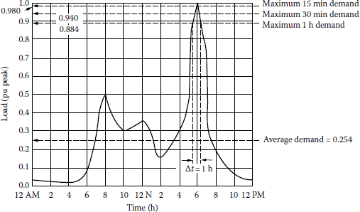
The demand statement should express the demand interval Δt used to measure it. Figure 2.1 shows a daily demand variation curve, or load curve, as a function of demand intervals. Note that the selection of both Δt and total time t is arbitrary. The load is expressed in per unit (pu) of peak load of the system. For example, the maximum of 15-min demands is 0.940 pu, and the maximum of 1-h demands is 0.884, whereas the average daily demand of the system is 0.254. The data given by the curve of Figure 2.1 can also be expressed as shown in Figure 2.2. Here, the time is given in per unit of the total time. The curve is constructed by selecting the maximum peak points and connecting them by a curve. This curve is called the load duration curve. The load duration curves can be daily, weekly, monthly, or annual. For example, if the curve is a plot of all the 8760 hourly loads during the year, it is called an annual load duration curve. In that case, the curve shows the individual hourly loads during the year, but not in the order that they occurred, and the number of hours in the year that load exceeded the value is also shown.

The hour-to-hour load on a system changes over a wide range. For example, the daytime peak load is typically double the minimum load during the night. Usually, the annual peak load is, due to seasonal variations, about three times the annual minimum.
To calculate the average demand, the area under the curve has to be determined. This can easily be achieved by a computer program.
Maximum demand: “The maximum demand of an installation or system is the greatest of all demands which have occurred during the specified period of time” [1]. The maximum demand statement should also express the demand interval used to measure it. For example, the specific demand might be the maximum of all demands such as daily, weekly, monthly, or annual.
Example 2.1
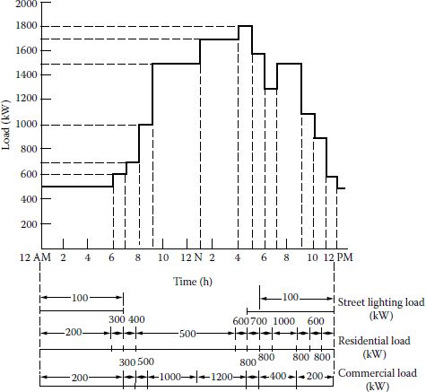
Assume that the loading data given in Table 2.1 belongs to one of the primary feeders of the No Light & No Power (NL&NP) Company and that they are for a typical winter day. Develop the idealized daily load curve for the given hypothetical primary feeder.
Idealized Load Data for the NL&NP’s Primary Feeder
Load, kW |
|||
|---|---|---|---|
Time |
Street Lighting |
Residential |
Commercial |
12 AM |
100 |
200 |
200 |
1 |
100 |
200 |
200 |
2 |
100 |
200 |
200 |
3 |
100 |
200 |
200 |
4 |
100 |
200 |
200 |
5 |
100 |
200 |
200 |
6 |
100 |
200 |
200 |
7 |
100 |
300 |
200 |
8 |
400 |
300 |
|
9 |
500 |
500 |
|
10 |
500 |
1000 |
|
11 |
500 |
1000 |
|
12 noon |
500 |
1000 |
|
1 |
500 |
1000 |
|
2 |
500 |
1200 |
|
3 |
500 |
1200 |
|
4 |
500 |
1200 |
|
5 |
600 |
1200 |
|
6 |
100 |
700 |
800 |
7 |
100 |
800 |
400 |
8 |
100 |
1000 |
400 |
9 |
100 |
1000 |
400 |
10 |
100 |
800 |
200 |
11 |
100 |
600 |
200 |
12 PM |
100 |
300 |
200 |
Solution
The solution is self-explanatory, as shown in Figure 2.3.
Diversified demand (or coincident demand): It is the demand of the composite group, as a whole, of somewhat unrelated loads over a specified period of time. Here, the maximum diversified demand has an importance. It is the maximum sum of the contributions of the individual demands to the diversified demand over a specific time interval.
For example, “if the test locations can, in the aggregate, be considered statistically representative of the residential customers as a whole, a load curve for the entire residential class of customers can be prepared. If this same technique is used for other classes of customers, similar load curves can be prepared” [3]. As shown in Figure 2.4, if these load curves are aggregated, the system load curve can be developed. The interclass coincidence relationships can be observed by comparing the curves.
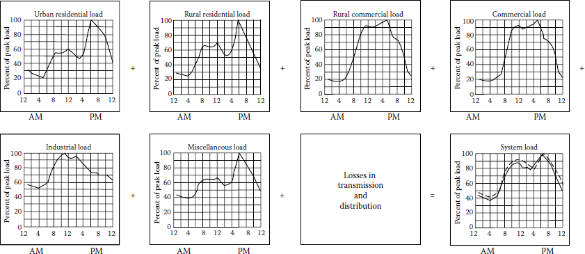
Development of aggregate load curves for winter peak period. Miscellaneous load includes street lighting and sales to other agencies. Dashed curve shown on system load diagram is actual system generation sent out. Solid curve is based on group load study data.
(From Sarikas, R.H. and Thacker, H.B., AIEE Trans., 31(pt. III), 564, August 1957. Used by permission.)
Noncoincident demand: Manning [2] defines it as “the sum of the demands of a group of loads with no restrictions on the interval to which each demand is applicable.” Here, again the maximum of the noncoincident demand is the value of some importance.
Demand factor: It is the “ratio of the maximum demand of a system to the total connected load of the system” [1]. Therefore, the demand factor (DF) is
DF≜Maximum demandTotal connected demand (2.1)
The DF can also be found for a part of the system, for example, an industrial or commercial customer, instead of for the whole system. In either case, the DF is usually less than 1.0. It is an indicator of the simultaneous operation of the total connected load.
Connected load: It is “the sum of the continuous ratings of the load-consuming apparatus connected to the system or any part thereof” [1]. When the maximum demand and total connected demand have the same units, the DF is dimensionless.
Utilization factor: It is “the ratio of the maximum demand of a system to the rated capacity of the system” [1]. Therefore, the utilization factor (Fu) is
Fu≜Maximum demandRated system capacity (2.2)
The utilization factor can also be found for a part of the system. The rated system capacity may be selected to be the smaller of thermal- or voltage-drop capacity [2].
Plant factor: It is the ratio of the total actual energy produced or served over a designated period of time to the energy that would have been produced or served if the plant (or unit) had operated continuously at maximum rating. It is also known as the capacity factor or the use factor. Therefore,
Plant factor=Actual energy produced or served ×TMaximum plant rating ×T (2.3)
It is mostly used in generation studies. For example,
Annual plant factor=Actual annual energy generationMaximum plant rating (2.4)
or
Annual plant factor=Actual annual energy generationMaximum plant rating × 8760 (2.5)
Load factor: It is “the ratio of the average load over a designated period of time to the peak load occurring on that period” [1]. Therefore, the load factor FLD is o average load:
FLD≜Average LoadPeak Load (2.6)
or
FLD≜Average load×TPeak load×T=Units servedPeak load×T (2.7)
where T is the time, in days, weeks, months, or years. The longer the period T, the smaller the resultant factor. The reason for this is that for the same maximum demand, the energy consumption covers a larger time period and results in a smaller average load. Here, when time T is selected to be in days, weeks, months, or years, use it in 24, 168, 730, or 8760 h, respectively. It is less than or equal to 1.0.
Therefore,
Annual load factor=Total annual energyAnnual peak load × 8760 (2.8)
Diversity factor: It is “the ratio of the sum of the individual maximum demands of the various subdivisions of a system to the maximum demand of the whole system” [1]. Therefore, the diversity factor (FD) is
FD≜Sum of individual maximum demandsCoincident maximum demand (2.9)
or
FD=D1+D2+D3+⋯+DnDg (2.10)
or
FD=∑ni=1DiDg (2.11)
where
Di is the maximum demand of load i, disregarding time of occurrence
Dg = D1+2+3+···+n
= coincident maximum demand of group of n loads
The diversity factor can be equal to or greater than 1.0.
From Equation 2.1,
DF=Maximum demandTotal connected demand
or
Maximum demand = Total connected demand × DF (2.12)
Substituting Equation 2.12 into 2.11, the diversity factor can also be given as
FD=∑ni=1TCDi×DFiDg (2.13)
where
TCDi is the total connected demand of group, or class, i load
DFi is the demand factor of group, or class, i load
Coincidence factor: It is “the ratio of the maximum coincident total demand of a group of consumers to the sum of the maximum power demands of individual consumers comprising the group both taken at the same point of supply for the same time” [1]. Therefore, the coincidence factor (Fc) is
Fc=Coincident maximum demandSum of individual maximum demands (2.14)
or
Fc=Dg∑ni=1Di (2.15)
Thus, the coincidence factor is the reciprocal of diversity factor, that is,
Fc=1FD (2.16)
These ideas on the diversity and coincidence are the basis for the theory and practice of north-to-south and east-to-west interconnections among the power pools in this country. For example, in the United States during winter, energy comes from south to north, and during summer, just the opposite occurs. Also, east-to-west interconnections help to improve the energy dispatch by means of sunset or sunrise adjustments, that is, the setting of clocks 1 h late or early.
Load diversity: It is “the difference between the sum of the peaks of two or more individual loads and the peak of the combined load” [1]. Therefore, the load diversity (LD) is
LD≜(n∑i=1Di)−Dg (2.17)
Contribution factor: Manning [2] defines ci as “the contribution factor of the ith load to the group maximum demand.” It is given in per unit of the individual maximum demand of the ith load. Therefore,
Dg≜c1×D1+c2×D2+c3×D3+⋯+cn×Dn (2.18)
Substituting Equation 2.18 into 2.15,
Fc=c1×D1+c2×D2+c3×D3+⋯+cn×Dn∑ni=1Di (2.19)
or
Fc=∑ni=1ci×Di∑ni=1Di (2.20)
Special cases
Case 1: D1 = D2 = D3 = ... = Dn = D. From Equation 2.20,
Fc=D×∑ni=1cin×D (2.21)
or
Fc=∑ni=1cin (2.22)
That is, the coincidence factor is equal to the average contribution factor.
Case 2: c1 = c2 = c3 = ... = cn = c. Hence, From Equation 2.20,
Fc=c×∑ni=1Di∑ni=1Di (2.23)
or
Fc=c (2.24)
That is, the coincidence factor is equal to the contribution factor.
Loss factor: It is “the ratio of the average power loss to the peak-load power loss during a specified period of time” [1]. Therefore, the loss factor (FLS) is
FLS≜Average power lossPower lossat peak load (2.25)
Equation 2.25 is applicable for the copper losses of the system but not for the iron losses.
Example 2.2
Assume that the annual peak load of a primary feeder is 2000 kW, at which the power loss, that is, total copper, or ∑I2Rloss, is 80 kW per three phase. Assuming an annual loss factor of 0.15, determine
- The average annual power loss
- The total annual energy loss due to the copper losses of the feeder circuits
Solution
- From Equation 2.25,
Average power loss=power loss at peak load×FLs=80kW×0.15=12kW
- The total annual energy loss is
TAELCu=average power loss × 8760 h/year=12×8760 = 105,120 kWh
Example 2.3
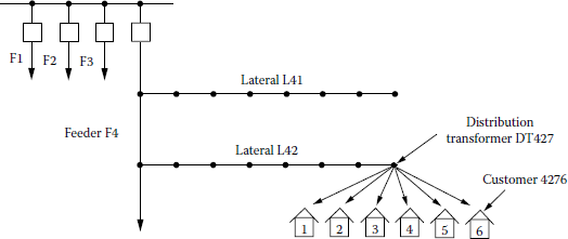
There are six residential customers connected to a distribution transformer (DT), as shown in Figure 2.5. Notice the code in the customer account number, for example, 4276. The first figure, 4, stands for feeder F4; the second figure, 2, indicates the lateral number connected to the F4 feeder; the third figure, 7, is for the DT on that lateral; and finally the last figure, 6, is for the house number connected to that DT.
Assume that the connected load is 9 kW per house and that the DF and diversity factor for the group of six houses, either from the NL&NP Company’s records or from the relevant handbooks, have been decided as 0.65 and 1.10, respectively. Determine the diversified demand of the group of six houses on the DT DT427.
Solution
From Equation 2.13, the diversified demand of the group on the DT is
Example 2.4
Assume that feeder 4 of Example 2.3 has a system peak of 3000 kVA per phase and a copper loss of 0.5% at the system peak. Determine the following:
- The copper loss of the feeder in kilowatts per phase
- The total copper losses of the feeder in kilowatts per three phase
Solution
- The copper loss of the feeder in kilowatts per phase is
- The total copper losses of the feeder in kilowatts per three phase is
Example 2.5
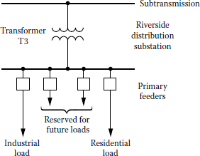
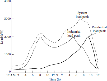
Assume that there are two primary feeders supplied by one of the three transformers located at the NL&NP’s Riverside distribution substation, as shown in Figure 2.6. One of the feeders supplies an industrial load that occurs primarily between 8 AM and 11 PM, with a peak of 2000 kW at 5 PM. The other one feeds residential loads that occur mainly between 6 AM and 12 PM, with a peak of 2000 kW at 9 PM, as shown in Figure 2.7. Determine the following:
- The diversity factor of the load connected to transformer T3
- The load diversity of the load connected to transformer T3
- The coincidence factor of the load connected to transformer T3
Solution
- From Equation 2.11, the diversity factor of the load is
- From Equation 2.17, the load diversity of the load is
- From Equation 3.16, the coincidence factor of the load is
Example 2.6
Use the data given in Example 2.1 for the NL&NP’s load curve. Note that the peak occurs at 4 PM. Determine the following:
- The class contribution factors for each of the three load classes
- The diversity factor for the primary feeder
- The diversified maximum demand of the load group
- The coincidence factor of the load group
Solution
- The class contribution factor is
For street lighting, residential, and commercial loads,
- From Equation 2.11, the diversity factor is
and from Equation 2.18,
Substituting Equation 2.18 into 2.11,
Therefore, the diversity factor for the primary feeder is
- The diversified maximum demand is the coincident maximum demand, that is, Dg. Therefore, from Equation 2.13, the diversity factor is
where the maximum demand, from Equation 2.12, is
Substituting Equation 2.12 into 2.13,
or
Therefore, the diversified maximum demand of the load group is
- The coincidence factor of the load group, from Equation 2.15, is
or, from Equation 2.16,
2.2 Relationship Between the Load and Loss Factors
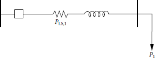
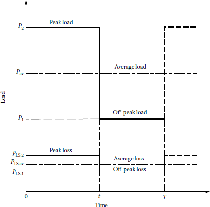
In general, the loss factor cannot be determined from the load factor. However, the limiting values of the relationship can be found [2]. Assume that the primary feeder shown in Figure 2.8 is connected to a variable load. Figure 2.9 shows an arbitrary and idealized load curve. However, it does not represent a daily load curve. Assume that the off-peak loss is PLS,1 at some off-peak load Pj and that the peak loss is PLS,2 at the peak load P2. The load factor is
From Figure 2.9,
Substituting Equation 2.27 into 2.26,
or
The loss factor is
where
PLS,av is the average power loss
PLS,max is the maximum power loss
PLS,2 is the peak loss at peak load
From Figure 2.9,
Substituting Equation 2.30 into 2.29,
where
PLS,1 is the off-peak loss at off-peak load
t is the peak-load duration
T – t is the off-peak-load duration
The copper losses are the function of the associated loads. Therefore, the off-peak and peak loads can be expressed, respectively, as
and
where k is a constant. Thus, substituting Equations 2.32 and 2.33 into 2.31, the loss factor can be expressed as
or
By using Equations 2.28 and 2.35, the load factor can be related to loss factor for three different cases.
Case 1: Off-peak load is zero. Here,
since P1 = 0. Therefore, from Equations 2.28 through 2.35,
That is, the load factor is equal to the loss factor, and they are equal to the tIT constant.
Case 2: Very short-lasting peak. Here,
hence in Equations 2.28 and 2.35,
therefore,
That is, the value of the loss factor approaches the value of the load factor squared.
Case 3: Load is steady. Here,
That is, the difference between the peak load and the off-peak load is negligible. For example, if the customer’s load is a petrochemical plant, this would be the case. Thus, from Equations 2.28 through 2.35,
That is, the value of the loss factor approaches the value of the load factor.
Therefore, in general, the value of the loss factor is
Therefore, the loss factor cannot be determined directly from the load factor. The reason is that the loss factor is determined from losses as a function of time, which, in turn, are proportional to the time function of the square load [2–4].
However, Buller and Woodrow [5] developed an approximate formula to relate the loss factor to the load factor as
where
FLS is the loss factor, pu
FLD is the load factor, pu
Equation 2.40a gives a reasonably close result. Figure 2.10 gives three different curves of loss factor as a function of load factor. Relatively recently, the formula given earlier has been modified for rural areas and expressed as
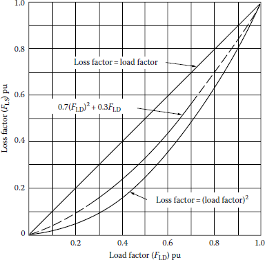
Loss factor curves as a function of load factor.
(From Westinghouse Electric Corporation, Electric Utility Engineering Reference Book-Distribution Systems, Vol. 3, Westinghouse Electric Corporation, East Pittsburgh, PA, 1965.)
Example 2.7
The average load factor of a substation is 0.65. Determine the average loss factor of its feeders, if the substation services
- An urban area
- A rural area
Solution
- For the urban area,
- For the rural area,
Example 2.8
Assume that the Riverside distribution substation of the NL&NP Company supplying Ghost Town, which is a small city, experiences an annual peak load of 3500 kW. The total annual energy supplied to the primary feeder circuits is 10,000,000 kWh. The peak demand occurs in July or August and is due to air-conditioning load.
- Find the annual average power demand.
- Find the annual load factor.
Solution
Assume a monthly load curve as shown in Figure 2.11.
- The annual average power demand is
- From Equation 2.6, the annual load factor is
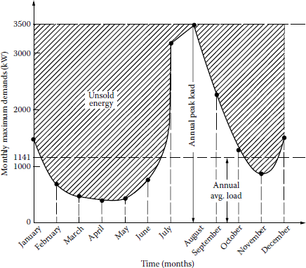
or, from Equation 2.8,
The unsold energy, as shown in Figure 2.11, is a measure of capacity and investment cost. Ideally, it should be kept at a minimum.
Example 2.9
Use the data given in Example 2.8 and suppose that a new load of 100 kW with 100% annual load factor is to be supplied from the Riverside substation. The investment cost, or capacity cost, of the power system upstream, that is, toward the generator, from this substation is $18.00/kW per month. Assume that the energy delivered to these primary feeders costs the supplier, that is, NL&NP, $0.06/kWh.
- Find the new annual load factor on the substation.
- Find the total annual cost to NL&NP to serve this load.
Solution
Figure 2.12 shows the new load curve after the addition of the new load of 100 kW with 100% load.
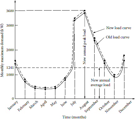
- The new annual load factor on the substation is
- The total annual and additional cost to NL&NP to serve the additional 100 kW load has two cost components, namely, (1) annual capacity cost and (2) annual energy cost. Therefore,
and
Therefore,
Example 2.10
Assume that the annual peak-load input to a primary feeder is 2000 kW. A computer program that calculates voltage drops and I2R losses shows that the total copper loss at the time of peak load is . The total annual energy supplied to the sending end of the feeder is 5.61 × 10⁶ kWh.
- By using Equation 2.40, determine the annual loss factor.
- Calculate the total annual copper loss energy and its value at $0.06/kWh.
Solution
- From Equation 2.40, the annual loss factor is
where
Therefore,
- From Equation 2.25,
or
Example 2.11
Assume that one of the DTs of the Riverside substation supplies three primary feeders. The 30 min annual maximum demands per feeder are listed in the following table, together with the power factor (PF) at the time of annual peak load.
Demand |
||
|---|---|---|
Feeder |
kW |
PF |
1 |
1800 |
0.95 |
2 |
2000 |
0.85 |
3 |
2200 |
0.90 |
Assume a diversity factor of 1.15 among the three feeders for both real power (P) and reactive power (Q).
- Calculate the 30 min annual maximum demand on the substation transformer in kilowatts and in kilovoltamperes.
- Find the load diversity in kilowatts.
- Select a suitable substation transformer size if zero load growth is expected and if company policy permits as much as 25% short-time overloads on the distribution substation transformers. Among the standard three-phase (3ϕ) transformer sizes available are the following:
2500/3125 kVA self-cooled/forced-air-cooled
3750/4687 kVA self-cooled/forced-air-cooled
5000/6250 kVA self-cooled/forced-air-cooled
7500/9375 kVA self-cooled/forced-air-cooled - Now assume that the substation load will increase at a constant percentage rate per year and will double in 10 years. If the 7500/9375 kVA-rated transformer is installed, in how many years will it be loaded to its fans-on rating?
Solution
- From Equation 2.10,
Therefore,
To find power in kilovoltamperes, find the PF angles. Therefore,
Thus, the diversified reactive power (Q) is
Therefore,
- From Equation 2.17, the load diversity is
- From the given transformer list, it is appropriate to choose the transformer with the 3750/4687-kVA rating since with the 25% short-time overload, it has a capacity of
which is larger than the maximum demand of 5793.60 kVA as found in part (a).
- Note that the term fans-on rating means the forced-air-cooled rating. To find the increase (g) per year,
(1 + g)10 = 2
hence,
1 + g = 1.07175
or
g = 7.175%/year
Thus,
(1.07175)n × 5793.60 = 9375 kVA
or
(1.07175)n = 1.6182
Therefore,
Therefore, if the 7500/9375 kVA-rated transformer is installed, it will be loaded to its fans-on rating in about 7 years.
2.3 Maximum Diversified Demand
Arvidson [7] developed a method of estimating DT loads in residential areas by the diversified-demand method, which takes into account the diversity between similar loads and the noncoincidence of the peaks of different types of loads.
To take into account the noncoincidence of the peaks of different types of loads, Arvidson introduced the hourly variation factor. It is “the ratio of the demand of a particular type of load coincident with the group maximum demand to the maximum demand of that particular type of load [2].” Table 2.2 gives the hourly variation curves for various types of household appliances. Figure 2.13 shows a number of curves for various types of household appliances to determine the average maximum diversified demand per customer in kilowatts per load. In Figure 2.13, each curve represents a 100% saturation level for a specific demand.
Hourly Variation Factors
Heat Pumpa |
||||||||||||
|---|---|---|---|---|---|---|---|---|---|---|---|---|
Hour |
Lighting and Miscellaneous Refrigerator |
Home Freezer |
Range |
Air-Conditioninga |
Cooling Season |
Heating Season |
Housea Heating |
Both Elements Restricted |
Only Bottom Elements Restricted |
Uncontrolled |
Clothesd Dryer |
|
12 AM |
0.32 |
0.93 |
0.92 |
0.02 |
0.40 |
0.42 |
0.34 |
0.11 |
0.41 |
0.61 |
0.51 |
0.03 |
1 |
0.12 |
0.89 |
0.90 |
0.01 |
0.39 |
0.35 |
0.49 |
0.07 |
0.33 |
0.46 |
0.37 |
0.02 |
2 |
0.10 |
0.80 |
0.87 |
0.01 |
0.36 |
0.35 |
0.51 |
0.09 |
0.25 |
0.34 |
0.30 |
0 |
3 |
0.09 |
0.76 |
0.85 |
0.01 |
0.35 |
0.28 |
0.54 |
0.08 |
0.17 |
0.24 |
0.22 |
0 |
4 |
0.08 |
0.79 |
0.82 |
0.01 |
0.35 |
0.28 |
0.57 |
0.13 |
0.13 |
0.19 |
0.15 |
0 |
5 |
0.10 |
0.72 |
0.84 |
0.02 |
0.33 |
0.26 |
0.63 |
0.15 |
0.13 |
0.19 |
0.14 |
0 |
6 |
0.19 |
0.75 |
0.85 |
0.05 |
0.30 |
0.26 |
0.74 |
0.17 |
0.17 |
0.24 |
0.16 |
0 |
7 |
0.41 |
0.75 |
0.85 |
0.30 |
0.41 |
0.35 |
1.00 |
0.76 |
0.27 |
0.37 |
0.46 |
0 |
8 |
0.35 |
0.79 |
0.86 |
0.47 |
0.53 |
0.49 |
0.91 |
1.00 |
0.47 |
0.65 |
0.70 |
0.08 |
9 |
0.31 |
0.79 |
0.86 |
0.28 |
0.62 |
0.58 |
0.83 |
0.97 |
0.63 |
0.87 |
1.00 |
0.20 |
10 |
0.31 |
0.79 |
0.87 |
0.22 |
0.72 |
0.70 |
0.74 |
0.68 |
0.67 |
0.93 |
1.00 |
0.65 |
11 |
0.30 |
0.85 |
0.90 |
0.22 |
0.74 |
0.73 |
0.60 |
0.57 |
0.67 |
0.93 |
0.99 |
1.00 |
12 noon |
0.28 |
0.85 |
0.92 |
0.33 |
0.80 |
0.84 |
0.57 |
0.55 |
0.67 |
0.93 |
0.98 |
0.98 |
i |
0.26 |
0.87 |
0.96 |
0.25 |
0.86 |
0.88 |
0.49 |
0.51 |
0.61 |
0.85 |
0.86 |
0.70 |
2 |
0.29 |
0.90 |
0.98 |
0.16 |
0.89 |
0.95 |
0.46 |
0.49 |
0.55 |
0.76 |
0.82 |
0.65 |
3 |
0.30 |
0.90 |
0.99 |
0.17 |
0.96 |
1.00 |
0.40 |
0.48 |
0.49 |
0.68 |
0.81 |
0.63 |
4 |
0.32 |
0.90 |
1.00 |
0.24 |
0.97 |
1.00 |
0.43 |
0.44 |
0.33 |
0.46 |
0.79 |
0.38 |
5 |
0.70 |
0.90 |
1.00 |
0.80 |
0.99 |
1.00 |
0.43 |
0.79 |
0 |
0.09 |
0.75 |
0.30 |
6 |
0.92 |
0.90 |
0.99 |
1.00 |
1.00 |
1.00 |
0.49 |
0.88 |
0 |
0.13 |
0.75 |
0.22 |
7 |
1.00 |
0.95 |
0.98 |
0.30 |
0.91 |
0.88 |
0.51 |
0.76 |
0 |
0.19 |
0.80 |
0.26 |
8 |
0.95 |
1.00 |
0.98 |
0.12 |
0.79 |
0.73 |
0.60 |
0.54 |
1.00 |
1.00 |
0.81 |
0.20 |
9 |
0.85 |
0.95 |
0.97 |
0.09 |
0.71 |
0.72 |
0.54 |
0.42 |
0.84 |
0.98 |
0.73 |
0.18 |
10 |
0.72 |
0.88 |
0.96 |
0.05 |
0.64 |
0.53 |
0.51 |
0.27 |
0.67 |
0.77 |
0.67 |
0.10 |
11 |
0.50 |
0.88 |
0.95 |
0.04 |
0.55 |
0.49 |
0.34 |
0.23 |
0.54 |
0.69 |
0.59 |
0.04 |
12 PM |
0.32 |
0.93 |
0.92 |
0.02 |
0.40 |
0.42 |
0.34 |
0.11 |
0.44 |
0.61 |
0.51 |
0.03 |
Source: From Sarikas, R.H. and Thacker, H.B., AIEE Trans., 31(pt. III), 564, August 1957. With permission.
a Load cycle and maximum diversified demand are dependent on outside temperature, dwelling construction and insulation, among other factors.
b Load cycle and maximum diversified demands are dependent on tank size, and heater element rating; values shown apply to 52 gal tank, 1500 and 1000 W elements.
c Load cycle dependent on schedule of water heater restriction.
d Hourly variation factor is dependent on living habits of individuals; in a particular area, values may be different from those shown. gn
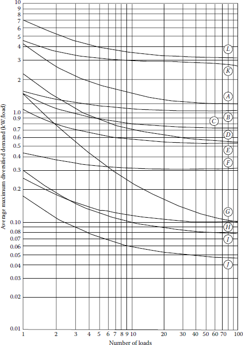
Maximum diversified 30 min demand characteristics of various residential loads: A, clothes dryer; B, off-peak water heater, “off-peak” load; C, water heater, uncontrolled, interlocked elements; D, range; E, lighting and miscellaneous appliances; F, 0.5-hp room coolers; G, off-peak water heater, “on-peak” load, upper element uncontrolled; H, oil burner; I, home freezer; J, refrigerator; K, central air-conditioning, including heat-pump cooling, 5-hp heat pump (4-ton air conditioner); L, house heating, including heat-pump-heating-connected load of 15 kW unit-type resistance heating or 5 hp heat pump.
(From Westinghouse Electric Corporation, Electric Utility Engineering Reference Book-Distribution Systems, Vol. 3, Westinghouse Electric Corporation, East Pittsburgh, PA, 1965.)
To apply Arvidson’s method to determine the maximum diversified demand for a given saturation level and appliance, the following steps are suggested [2]:
- Determine the total number of appliances by multiplying the total number of customers by the per-unit saturation.
- Read the corresponding diversified demand per customer from the curve, in Figure 2.13, for the given number of appliances.
- Determine the maximum demand, multiplying the demand found in step 2 by the total number of appliances.
- Finally, determine the contribution of that type load to the group maximum demand by multiplying the resultant value from step 3 by the corresponding hourly variation factor found from Table 2.2.
Example 2.12
Assume a typical DT that serves six residential loads, that is, houses, through six service drops (SDs) and two spans of secondary line (SL). Suppose that there are a total of 150 DTs and 900 residences supplied by this primary feeder. Use Figure 2.13 and Table 2.2. For the sake of illustration, assume that a typical residence contains a clothes dryer, a range, a refrigerator, and some lighting and miscellaneous appliances. Determine the following:
- The 30 min maximum diversified demand on the DT.
- The 30 min maximum diversified demand on the entire feeder.
- Use the typical hourly variation factors given in Table 2.2 and calculate the small portion of the daily demand curve on the DT, that is, the total hourly diversified demands at 4, 5, and 6 PM, on the DT, in kilowatts.
Solution
- To determine the 30 min maximum diversified demand on the DT, the average maximum diversified demand per customer is found from Figure 2.13. Therefore, when the number of loads is six, the average maximum diversified demands per customer are
Thus,
and for six houses
(3.076 kW/house)(6 houses) = 18.5 kW
Thus, the contributions of the appliances to the 30 min maximum diversified demand on the DT is approximately 18.5 kW.
- As in part (a), the average maximum diversified demand per customer is found from Figure 2.13. Therefore, when the number of loads is 900 (note that, due to the given curve characteristics, the answers would be the same as the ones for the number of loads of 100), then the average maximum diversified demands per customer are
Hence,
Therefore, the 30 min maximum diversified demand on the entire feeder is
However, if the answer for the 30 min maximum diversified demand on one DT found in part (a) is multiplied by 150 to determine the 30 min maximum diversified demand on the entire feeder, the answer would be
150 × 18.5 ≅ 2775 kW
which is greater than the demand 2064.6 kW found previously. This discrepancy is due to the application of the appliance diversities.
- From Table 2.2, the hourly variation factors can be found as 0.38, 0.24, 0.90, and 0.32 for dryer, range, refrigerator, and lighting and miscellaneous appliances. Therefore, the total hourly diversified demands on the DT can be calculated as given in the following table in which
(1.6 kW/house)(6 houses)
= 9.6 kW
(0.8 kW/house)(6 houses)
= 4.8 kW
(0.066 kW/house)(6 houses)
= 0.4 kW
(0.61 kW/house)(6 houses)
= 3.7 kW
Lighting and Misc.
Total Hourly
Time
Dryers, kW
Ranges, kW
Refrigerators, kW
Appliances, kW
Diversified Demand, kW
(1)
(2)
(3)
(4)
(5)
(6)
4 PM
9.6 × 0.38
4.8 × 0.24
0.4 × 0.90
3.7 × 0.32
6.344
5 PM
9.6 × 0.30
4.8 × 0.80
0.4 × 0.90
3.7 × 0.70
9.670
6 PM
9.6 × 0.22
4.8 × 1.00
0.4 × 0.90
3.7 × 0.92
10.674
Note: The results given in column (6) are the sum of the contributions to demand given in columns (2)–(5).
2.4 Load Forecasting
The load growth of the geographical area served by a utility company is the most important factor influencing the expansion of the distribution system. Therefore, forecasting of load increases is essential to the planning process.
Fitting trends after transformation of data is a common practice in technical forecasting. An arithmetic straight line that will not fit the original data may fit, for example, the logarithms of the data as typified by the exponential trend
This expression is sometimes called a growth equation, since it is often used to explain the phenomenon of growth through time. For example, if the load growth rate is known, the load at the end of the nth year is given by
where
Pn is the load at the end of the nth year
P0 is the initial load
g is the annual growth rate
n is the number of years
Now, if it is set so that Pn = yt, P0 = a, 1 + g = b, and n = x, then Equation 2.42 is identical to the exponential trend equation (2.41). Table 2.3 gives a MATLAB® computer program to forecast the future demand values if the past demand values are known.
MATLAB® Demand-Forecasting Computer Program
%RLXD = read past demand values in MW
%RLXC = predicted future demand values in MW
%NP = number of years in the past up to the present
%NF = number of years from the present to the future that will be predicted
NP = input(‘Enter the number of years in the past up to the present:’);
NF = input(‘Enter the number of years from the present to the future that will be predicted:’);
for I = 1:NP
fprintf(‘Enter the past demand values in MW:" I); RLXD(I) = input(");
end
SXIYI = 0; SXISQ = 0; SXI = 0; SYI = 0; SYISQ = 0;
for I = I:NP XI = I-I;
Y(I) = 10g(RLXD(I)); SXIYI = SXIYI+XI*Y(I); SXI = SXI+X1; SY1 = SY1+ Y (I); SXISQ = SXISQ+ XI/2; SY1SQ = SY1SQ+ Y(1)A2;
end
A = (SXIY1-(SXI*SY1)/NP)/(SXISQ-(SXI/2)/NP); B = SYI/NP-A *SXI/NP;
R = exp(A);
RLXC(1) = exp(B);
RG = R-l;
fprintf(‘

Rate of growth =%f

’, RG);
NN = NP+NF;
for I = 2:NN XI = I-I;
DY = A * XI + B; RLXC(I) = exp(DY);
end
fprintf(‘	RLXD		RLXC
’); for I = I:NP
fprintf(‘	%f	%f
’, RLXD(I), RLXC(I)); end’
for I = I:NF
IP = I + NP; fprintf(‘				%f
’, RLXC(IP)); end
|
In order to plan the resources required to supply the future loads in an area, it is necessary to forecast the magnitude and distribution of these loads as accurately as possible. Such forecasts are normally based upon projections of the historical growth trend for the area and the existing load distribution within the area. Adjustments must be made for load transfers into and out of the area and for the addition or removal of block loads that are too large to be considered part of normal growth.
Before the 1973–1974 oil embargo, an exponential projection of adjusted historical peak loads provided satisfactory load forecasts for most distribution study areas. The growth in customers was reasonably steady, and the demand per customer continued to increase. However, in recent years, the picture has drastically changed. Energy conservation, load management, increasing electric rates, and a slow economy have combined to slow the growth. As a result, an exponential growth rate, such as the one given in the first part of this section, is no longer valid in most study areas.
Methods that forecast future demand by location divide the utility service area into a set of small areas forecasting the load growth in each. Most modern small-area forecast methods work with a uniform grid of small areas that covers the utility service area, as explained in Section 1.3.1, but the more traditional approach was to forecast the growth on a substation-by-substation or feeder-byfeeder basis, letting equipment service areas implicitly define the small areas.
Regardless of how small areas are defined, most forecasting methods themselves invariably fall into one of two categories, trending or land use. Trending methods extrapolate past historical peak loads using curve fitting or some other methods.
Contrarily, the behavior of load growth, in any relatively small area (served by substation, or feeder), is not a smooth curve, but is more like a sharp Gompertz curve, commonly referred to as an “S” curve. The S curve exhibits the distinct phases, namely, dormant, growth, and saturation phases. In the dormant phase, the small area has no load growth. In the growth phase, the load growth happens at a relatively rapid rate, usually due to new construction. In the saturation phase, the small area is fully developed. Any increase in load growth is extremely small.
By contrast, land-use simulation involves mapping existing and likely additions to land coverage by customer class definitions like residential, commercial, and industrial, in order to forecast growth. Either way, the ultimate goal is to project changes in the density of peak demand on a locality basis.
In order to plan a T&D system, it is necessary not just to study overall load in a region, but to study and forecast load on a spatial basis, that is, analyzing it in total and on a local area basis throughout the system, determining the where aspect of the load growth as well as the how much. Both are essential for determining T&D expansion needs.
Trend (or regression analysis) is the study of the behavior of a time series or a process in the past and its mathematical modeling so that future behavior can be extrapolated from it. Two usual approaches followed for trend analysis are
- The fitting of continuous mathematical functions through actual data to achieve the least overall error, known as regression analysis
- The fitting of a sequence on discontinuous lines or curves to the data
The second approach is more widespread in short-term forecasting. A time-varying event such as distribution system load can be broken down into the following four major components:
- Basic trend.
- Seasonal variation, that is, monthly or yearly variation of load.
- Cyclic variation that includes influences of periods longer than that provided earlier and causes the load pattern to be repeated for 2 or 3 years or even longer cycles.
- Random variations that occur on account of the day-to-day changes and in the case of power systems are usually dependent on weather and the time of the week, for example, weekday and weekend.
The principle of regression theory is that any function y = f(x) can be fitted to a set of points (x1, y1), (x2, y2) so as to minimize the sum of errors squared to each point, that is,
Sum of squared errors is used as it gives a significant indication of goodness of fit. Typical regression curves used in power system forecasting are
Linear |
y = a + bx |
Exponential |
y = a(1 + b)x |
Power |
y = axb |
Polynomial |
y = a + bx + cx2 |
Gompertz |
|
The coefficients used in these equations are called regression coefficients. The following are some of the methodologies used in applying some of the regression curves provided earlier:
Linear regression: It is applied by using the method of least squares. Here, the line y = a + bx is fitted to the sets of points (x1, y1), (x2, y2), ..., (xn, yn), that is,
By taking partial differentiation with respect to the regression coefficients and setting the resultant equations to zero to achieve the minimum error criterion,
and
The earlier process is also referred to as the least square line method.
Least square parabola: The parabola curve of y = a + bx + cx2 is fitted to minimize the sum of squared errors, that is,
By taking partial differentiation with respect to the regression coefficients and setting the resultant equations to zero give simultaneous equations that can be solved for a, b, and c coefficients.
Least square exponential: Here, the same approach that has been used in linear regression can be used at first, but is replaced by in Equations 2.43 and 2.44, and the regression coefficients are found. The resultant coefficients are then transformed back.
Multiple regression: Two or more variables can be treated by an extension of the same principle. For example, if an equation of z = a + bx + cy is required to fit to a series of points (x1, y1, z1), (x2, y2, z2),... then this is a multiple linear regression. Multi-nonlinear regressions are also used. Just like before, set the sum of squared errors,
then differentiate it with respect to a, b, and c so that one can get the following three simultaneous equations:
which can be solved for a, b, and c.
2.4.1 Box–Jenkins Methodology
This method uses a stochastic time series to forecast future load demands. It is a popular method for short-term (5 years or less) forecasting. Box and Jenkins [8] developed this method of forecasting by trying to account for repeated movements in the historical series (those movements comprising a trend), leaving a series made up of only random, that is, irregular movements. To model the systematic patterns inherent in this series, the method relies upon autoregressive and moving average processes to account for cyclical movements and upon differencing to account for seasonal and secular movements. The Box–Jenkins methodology is an iterative procedure by which a stochastic model is constructed. The process starts from the most simple structure with the least number of parameters and develops into as complex a structure as necessary to obtain an adequate model, in the sense of yielding white noise only [9].
2.4.2 Small-Area Load Forecasting
In this type of forecasting, the utility service area is divided into a set of small areas, and the future load growth in each area is forecasted. Most modern small-area forecast methods work with a uniform grid of small area that covers the utility service area, but the more traditional approach was to forecast growth on a substation-by-substation or feeder-by-feeder basis, letting equipment service areas implicitly define the small areas. Regardless of how small areas are defined, most forecasting methods are based on trending or land use.
Trending methods have been explained in Section 2.5; by contrast, land-use simulation involves mapping existing and likely additions to land coverage by customer class definitions like residential, commercial, and industrial, in order to forecast future growth. In either way, the final goal is to project changes in the density of peak demand on a locality basis.
According to Willis [10], small-area growth is not a smooth, continuous process from year to year. Instead, growth in a small area is intense for several years, then drops to very low levels while high growth suddenly begins in other areas. This led to the characterization of small-area growth with Gompertz or the S curve. Its use does not imply that small-area growth always follows an S-shaped load history, but only that there is seldom a middle ground between high and low growth rates.
Therefore, small-area forecasting is less a process of extrapolating trends; it is a determination of when small areas transition among zero, high, and low growth states. Land-use methods are much better at predicting such growth-state transitions. Furthermore, the forecaster gets better and more meaningful answers to “what-if?” type questions by using land-use-based simulation methods.
2.4.3 Spatial Load Forecasting
In general, small-area load growth is a spatial process. Also the majority of load growth effects in any small area are due to effects from other small areas, some very far away, and a function of the distances to those areas. Therefore, the forecast of any one area must be based upon an assessment data not only for that area, but also for many other neighboring areas.
The best available trending method in terms of tested accuracy is load-trend-coupled (LTC) extrapolation, using a modified form of Markov regression, in which the peak-load histories of up to several hundred small areas are extrapolated in a single computation, with the historical trend in each area influencing the extrapolation of others.
The influence of one area’s trend on other’s is found by using pattern recognition as another’s is found by using pattern recognition as a function of past trends and locations, making LTC trending a true spatial method. Its main advantage is economy of use. Only the peak-load histories of substations and feeders and X–Y locations of substations are required as input [10].
Figure 2.14 illustrates this method. It works with land-use classes that correspond to utility rate classes, differentiating electric consumption within each by end-use category, for example, heating, lighting, using peak day load curves on a 15 min demand-period basis. It is applied on a grid basis, with a spatial resolution of 2.5 acres (square areas 1/16 miles across). Base spatial data include multispectral satellite imagery of the region, used for land-use identification and mapping purposes, customer/billing/rate class data, end-use load curve and load research surveys, and metered load curve readings by substation throughout the system.
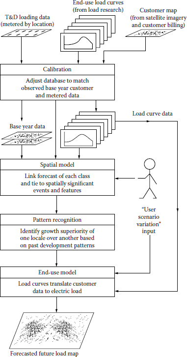
Spatial load forecasting.
(From Willis, H.L., Spatial Electric Load Forecasting, Marcel Dekker, New York, 1996.)
There are two inputs that control the forecast. The first one is the utility system-wide rate and marketing forecast. The second one is an optional set of scenario descriptors that allow the user to change future conditions to answer “what-if?” questions. It is very important that the base year model must provide accurately all known readings about customers, customer density, metered load curves, and their simultaneous variations in location and time.
Example 2.13
Write a simple MATLAB demand forecasting computer program based on the least-square exponential.
Solution
The MATLAB demand forecasting computer program is given in Table 2.4:
Demand Forecasting MATLAB Program
%%%%%%%%%%%%%%%%%%%%%%%%%%%%%%%%%%%%%%%%%%%%%%%%%%%%%%%%%%%%%%%%%
% demand forecasting matlab program
%%%%%%%%%%%%%%%%%%%%%%%%%%%%%%%%%%%%%%%%%%%%%%%%%%%%%%%%%%%%%%%%%%
fprintf(‘
Demand Forecast
’);
fprintf(‘
Enter an array of demand values in the form:
’);
fprintf(‘	[yr1 ld1; yr2 ld2; yr3 ld3; yr4 ld4; yr5 ld5]
’);
past_dem = input(‘
Enter year/demand values: ’);
sizepd = size(past_dem);
% get the # of past years of data and the # of cols in the array np = sizepd(1); cols = sizepd(2);
% get the number of years to predict
nf = input(‘
Enter the number of year to predict: ’);
ntotal = np + nf;
% obtain the least-square terms to estimate the ld growth value g
% y = ab^x must be transformed to ln(y) = ln(a) + x*ln(b)
Y = log(past_dem(:,2))’; X = 0:np - 1;
sumx2 = (X - mean(X))*(X - mean(X))’;
sumxy = (Y - mean(Y))*(X - mean(X))’;
% get the coeffs of the transformed data A = ln(b) and B = ln(a)
A = sumxy/sumx2; B = mean(Y) - A*mean(X);
% solve for the initial value, Po and g
Po = exp(B);
g = exp(A) - 1;
fprintf(‘
	Rate of growth =%2.2f%%

’, g*100);
fprintf(‘	YEAR	ACTUAL		FORECAST
’);
% calculate the estimated values
est_dem = 0;
for i = 1:ntotal
n = i - 1;
% year = first year + n
est_dem(i, 1) = past_dem(1, 1) + n;
% load growth equation
est_dem(i, 2) = Po*(1+g)^n;
if i < = np
 fprintf(‘	%4d	%6.2f		%6.2f
’, est_dem(i,1),past_dem(i,2),est_ dem(i,2));
else
 fprintf(‘	%4d	-			%6.2f
’, est_dem(i,1),est_dem(i,2));
end
end
plot(past_dem(:,1),past_dem(:,2), ‘k-s’, est_dem(:,1), est_dem(:,2), ‘k-+’);
xlabel(‘Year’); ylabel(‘Demand’); legend(‘Actual’, ‘Forecast’);
|
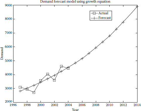
Example 2.14
Assume the peak MW July demands for the last 8 years have been the following: 3094, 2938, 2714, 3567, 4027, 3591, 4579, and 4436. Use the MATLAB program given in Example 2.13 as a curve-fitting technique and determine the following:
- The average rate of growth of the demand.
- Find out the ideal data based on growth for the past 8 years to give the correct demand forecast.
- The forecasted future demands for the next 10 years.
- Plot the results found in parts (a) and (b).
Solution
Here is the program output showing the answers for the parts (a) through (c). The answer for part (d) is given in Figure 2.15.
Program Output
EDU» load_growth
Demand Forcast
Enter an array of demand values in the following form:
[yr1 Id1; yr2 Id2; yr3 Id3; yr4 Id4; yr5 Id5; yr6 Id6; yr7 Id7]
An example is shown below:
[1997 3094; 1998 2938; 1999 2714; 2000 3567; 2001 4027; 2002
3591; 2003 4579]
Enter year/demand values: [1997 3094; 1998 2938; 1999 2714; 2000 3567;
2001 4027; 2002 3591; 2003 4579; 2004 4436]
Enter the number of year to predict: 10
Rate of growth = 5.55% |
||
YEAR |
ACTUAL |
FORECAST |
1997 |
3094 |
3094 |
1998 |
2938 |
3266 |
1999 |
2714 |
3447 |
2000 |
3567 |
3639 |
2001 |
4027 |
3841 |
2002 |
3591 |
4054 |
2003 |
4579 |
4279 |
2004 |
4436 |
4516 |
2005 |
– |
4767 |
2006 |
– |
5032 |
2007 |
– |
5311 |
2008 |
– |
5606 |
2009 |
– |
5918 |
2010 |
– |
6246 |
2011 |
– |
6593 |
2012 |
– |
6959 |
2013 |
– |
7345 |
2014 |
– |
7753 |
2015 |
– |
8184 |
EDU»
2.5 Load Management
The load management process involves controlling system loads by remote control of individual customer loads. Such control includes suppressing or biasing automatic control of cycling loads, as well as load switching. Load management can also be affected by inducing customers to suppress loads during utility-selected daily periods by means of time-of-day rate incentives. Such activities are called demand-side management.
Demand-side management (DSM): It includes all measures, programs, equipment, and activities that are directed toward improving efficiency and cost-effectiveness of energy usage on the customer side of the meter.
In general, such load control results in a load reduction at time t, that is, ΔS(t), that can be expressed as
where
Sav is the average connected load of controlled devices
Duncont (t) is the average duty cycle of uncontrolled units at time t
Dcont (t) is the duty cycle allowed by the load control at time t
N is the number of units under control
Distribution automation provides the control and monitoring ability required for both load management scenarios. It provides for direct control of customer loads and the monitoring necessary to verify that programmed levels are achieved. It also provides for the appropriate selection of energy metering registers where time-of-use rates are in effect.
The use of load management provides various benefits to the utility and its customers. Maximizing utilization of existing distribution system can lead to deferrals of capital expenditures. This is achieved by shaping the daily (monthly, annual) load characteristic in the following manner:
- By suppressing loads at peak times and/or encouraging energy consumption at off-peak times
- By minimizing the requirement for more costly generation or power purchases by suppressing loads
- By relieving the consequences of significant loss of generation or similar emergency situations by suppressing loads
- By reducing cold load pickup during reenergization of circuits using devices with cold load pickup features
Load management monitoring and control functions include the following:
- Monitoring of substations and feeder loads: To verify that the required magnitude of load suppression is accomplished for normal and emergency conditions as well as switch status
- Controlling individual customer loads: To suppress total system, substation, or feeder loads for normal or emergency conditions, and switching meter registers in order to accommodate time of use, that is, time of day, rate structures, where these are in effect
The effectiveness of direct control of customer loads is increased by choosing the larger and more significant customer loads. These include electric space and water heating, air-conditioning, electric clothes dryers, and others.
Also customer-activated load management is achieved by incentives such as time-of-use rates or customer alert to warn customers so that they can alter their use. In response to the economic penalty in terms of higher energy rates, the customers will limit their energy consumption during peak-load periods. Distribution automation provides for remotely adjusting and reading the time-of-use meters.
Example 2.15
Assume that a 5 kW air conditioner would run 80% of the time (80% duty cycle) and, during the peak hour, might be limited by utility remote control to a duty cycle of 65%. Determine the following:
- The number of minutes of operation denied at the end of 1 h of control of the unit
- The amount of reduced energy consumption during the peak hour if such control is applied simultaneously to 100,000 air conditioners throughout the system
- The total amount of reduced energy consumption during the peak
- The total amount of additional reduction in energy consumption in part (c) if T&D losses of the T&D system at peak is 8%
Solution
- The number of minutes of operation denied is
(0.80 – 0.65) × (60 min/h) = 9 min
- The amount of reduced energy consumption during the peak is
(0.80 – 0.65) × (5 kW) = 0.75 kW
- The total amount of energy reduction for 100,000 units is
- The total additional amount of energy reduction due to the reduction in the T&D losses is
(75 MW) × 0.08 = 6 MW
Thus, the overall total reduction is
75 MW + 6 MW = 81 MW
The earlier example shows attractiveness of controlling air conditioners to utility company.
2.6 Rate Structure
Even after the so-called deregulation, most public utilities are monopolies, that is, they have the exclusive right to sell their product in a given area. Their rates are subject to government regulation. The total revenue that a utility may be authorized to collect through the sales of its services should be equal to the company’s total cost of service. Therefore,
The determination of the revenue requirement is a matter of regulatory commission decision. Therefore, designing schedules of rates that will produce the revenue requirement is a management responsibility subject to commission review. However, a regulatory commission cannot guarantee a specific rate of earnings; it can only declare that a public utility has been given the opportunity to try to earn it.
The rate of return is partly a function of local conditions and should correspond with the return being earned by comparable companies with similar risks. It should be sufficient to permit the utility to maintain its credit and attract the capital required to perform its tasks.
However, the rate schedules, by law, should avoid unjust and unreasonable discrimination, that is, customers using the utility’s service under similar conditions should be billed at similar prices. It is a matter of necessity to categorize the customers into classes and subclasses, but all customers in a given class should be treated the same. There are several types of rate structures used by the utilities, and some of them are
- Flat demand rate structure
- Straight-line meter rate structure
- Block meter rate structure
- Demand rate structure
- Season rate structure
- Time-of-day (or peak-load pricing) structure
The flat rate structure provides a constant price per kilowatthour, which does not change with the time of use, season, or volume. The rate is negotiated knowing connected load; thus metering is not required. It is sometimes used for parking lot or street lighting service. The straight-line meter rate structure is similar to the flat structure. It provides a single price per kilowatthour without considering customer demand costs.
The block meter rate structure provides lower prices for greater usage, that is, it gives certain prices per kilowatthour for various kilowatthour blocks where the price per kilowatthour decreases for succeeding blocks. Theoretically, it does not encourage energy conservation and off-peak usage. Therefore, it causes a greater than necessary peak and, consequently, excess idle generation capacity during most of the time, resulting in higher rates to compensate the cost of a greater peak-load capacity.
The demand rate structure recognizes load factor and consequently provides separate charges for demand and energy. It gives either a constant price per kilowatthour consumed or a decreasing price per kilowatthour for succeeding blocks of energy used.
The seasonal rate structure specifies higher prices per kilowatthour used during the season of the year in which the system peak occurs (on-peak season) and lower prices during the season of the year in which the usage is the lowest (off-peak season).
The time-of-day rate structure (or peak-load pricing) is similar to the seasonal load rate structure. It specifies higher prices per kilowatthour used during the peak period of the day and lower prices during the off-peak period of the day.
The seasonal rate structure and the time-of-day rate structure are both designed to reduce the system’s peak load and therefore reduce the system’s idle standby capacity.
2.6.1 Customer Billing
Customer billing is done by taking the difference in readings of the meter at two successive times, usually at an interval of 1 month. The difference in readings indicates the amount of electricity, in kilowatthours, consumed by the customer in that period. This amount is multiplied by the appropriate rate or the series of rates and the adjustment factors, and the bill is sent to the customer.
Figure 2.16 shows a typical monthly bill rendered to a residential customer. The monthly bill includes the following items in the indicated spaces:
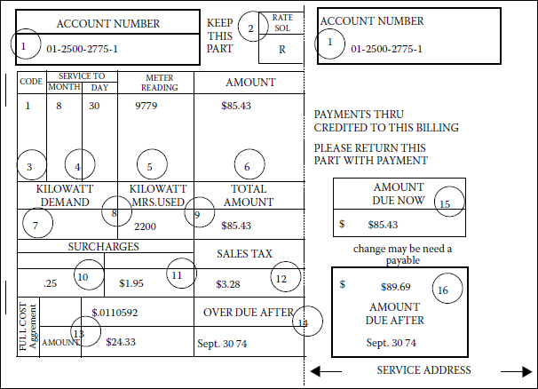
- The customer’s account number.
- A code showing which of the rate schedules was applied to the customer’s bill.
- A code showing whether the customer’s bill was estimated or adjusted.
- Date on which the billing period ended.
- Number of kilowatthours the customer’s meter registered when the bill was tabulated.
- Itemized list of charges. In this case, the only charge shown in box 6 of Figure 2.14 is a figure determined by adding the price of the electricity the customer has used to the routine taxes and surcharges. However, had the customer received some special service during this billing period, a service charge would appear in this space as a separate entry.
- Information appears in this box only when the bill is sent to a nonresidential customer using more than 6000 kWh electricity a month.
- The number of kilowatthours the customer used during the billing period.
- Total amount that the customer owes.
- Environmental surcharge.
- County energy tax.
- State sales tax.
- Fuel cost adjustment. Both the total adjustment and the adjustment per kilowatthour are shown.
- Date on which bill, if unpaid, becomes overdue.
- Amount due now.
- Amount that the customer must pay if the bill becomes overdue.
The sample electrical bill, shown in Figure 2.16, is based on the following rate schedule. Note that there is a minimum charge regardless of how little electricity the customer uses and that the first 20 kWh that the customer uses is covered by this flat rate. Included in the minimum, or service, charge is the cost of providing service to the customer, including metering, meter reading, billing, and various overhead expenses.
Rate schedule
Minimum Charge (Including First 20 kWh or Fraction Thereof) |
$2.25/month |
|---|---|
Next 80 kWh |
$0.0355/kWh |
Next 100 kWh |
$0.0321/kWh |
Next 200 kWh |
$0.0296/kWh |
Next 400 kWh |
$0.0265/kWh |
Consumption in excess of 800 kWh |
$0.0220/kWh |
The sample bill shows a consumption of 2200 kWh, which has been billed according to the following schedule:
First 20 kWh @ $2.25 (flat rate) |
= $2.25 |
Next 80 kWh × 0.0355 |
= $2.84 |
Next 100 kWh × 0.0321 |
= $3.21 |
Next 200 kWh × 0.096 |
= $5.92 |
Next 400 kWh × 0.0265 |
= $10.60 |
Additional 1400 kWh × 0.0220 |
= $30.80 |
2200 kWh |
= $55.62 |
Environmental surcharge |
= $0.25 |
County energy tax |
= $1.95 |
Fuel cost adjustment |
= $24.33 |
State sales tax |
= $3.28 |
Total amount |
= $85.43 |
Typical Energy Rate Schedule for Commercial Users
On-peak season (June 1–October 31) |
|
First 50 kWh or less/month for |
$4.09 |
Next 50 kWh/month |
@5.5090/kWh |
Next 500 kWh/month |
@4.8430/kWh |
Next 1400 kWh/month |
@4.0490/kWh |
Next 3000 kWh/month |
@3.8780/kWh |
All additional kWh/month |
@3.3390/kWh |
Off-peak season (November 1–May 31) |
|
First 50 kWh or less/month for |
4.09 |
Next 50 kWh/month |
@5.5090/kWh |
Next 500 kWh/month |
@4.2440/kWh |
Next 1400 kWh/month |
@3.1220/kWh |
Next 3000 kWh/month |
@2.7830/kWh |
All additional kWh/month |
@2.6490/kWh |
The customer is billed according to the utility company’s rate schedule. In general, the rates vary according to the season. In most areas, the demand for electricity increases in the warm months. Therefore, to meet the added burden, electric utilities are forced to use spare generators that are often less efficient and consequently more expensive to run. As an example, Table 2.5 gives a typical energy rate schedule for the on-peak and off-peak seasons for commercial users.
2.6.2 Fuel Cost Adjustment
The rates stated previously are based upon an average cost, in dollars per million Btu, for the cost of fuel burned at the NL&NP’s thermal generating plants. The monthly bill as calculated under the previously stated rate is increased or decreased for each kilowatthour consumed by an amount calculated according to the following formula:
where
FCAF is the fuel cost adjustment factor, $/kWh, to be applied per kilowatthour consumed
A is the weighted average Btu per kilowatthour for net generation from the NL&NP’s thermal plants during the second calendar month preceding the end of the billing period for which the kilowatthour usage is billed
B is the amount by which average cost of fuel per million Btu during the second calendar month preceding the end of the billing period for which the kilowatthour usage is billed exceeds or is less than $1/million Btu
C is the ratio, given in decimal, of the total net generation from all the NL&NP’s thermal plants during the second calendar month preceding the end of the billing period for which the kilo-watthour usage is billed to the total net generation from all the NL&NP’s plants including hydro generation owned by the NL&NP, or kilowatthours produced by hydro generation and purchased by the NL&NP, during the same period
D is the loss factor, which is the ratio, given in decimal, of kilowatthour losses (total kilowatthour losses less losses of 2.5% associated with off-system sales) to net system input, that is, total system input less total kilowatthours in off-system sales, for the year ending December 31 preceding; this ratio is updated every year and applied for 12 months
Example 2.16
Assume that the NL&NP Utility Company has the following, and typical, commercial rate schedule:
- Monthly billing demand = 30 min monthly maximum kilowatt demand multiplied by the ratio of (0.85/monthly average PF). The PF penalty shall not be applied when the consumer’s monthly average PF exceeds 0.85.
- Monthly demand charge = $2.00/kW of monthly billing demand.
- Monthly energy charges shall be as follows:
2.50 cents/kWh for the first 1000 kWh 2.00 cents/kWh for the next 3000 kWh
1.50 cents/kWh for all kWh in excess of 4000 - The total monthly charge shall be the sum of the monthly demand charge and the monthly energy charge.
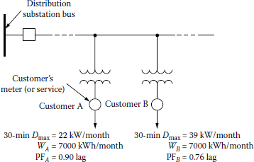
Assume that two consumers, as shown in Figure 2.17, each requiring a DT, are supplied from a primary line of the NL&NP.
- Assume that an average month is 730 h and find the monthly load factor of each consumer.
- Find a reasonable size, that is, continuous kilovoltampere rating, for each DT.
- Calculate the monthly bill for each consumer.
- It is not uncommon to measure the average monthly PF on a monthly energy basis, where both kilowatthours and kilovarhours are measured. On this basis, what size capacitor, in kilovars, would raise the PF of customer B to 0.85?
- Secondary-voltage shunt capacitors, in small sizes, may cost about $30/kvar installed with disconnects and short-circuit protection. Consumers sometimes install secondary capacitors to reduce their billings for utility service. Using the 30/kvar figure, find the number of months required for the PF correction capacitors found in part (d) to pay back for themselves with savings in demand charges.
Solution
- From Equation 2.7, the monthly load factors for each consumer are the following. For customer A,
and for customer B,
- The continuous kilovoltamperes for each DT are the following:
and
Therefore, the continuous sizes suitable for the DTs A and B are 25 and 50 kVA ratings, respectively.
- The monthly bills for each customer are the following:
For customer A
Monthly energy charge
First 1000 kWh = $0.025/kWh × 1000 kWh
= $25
Next 3000 kWh = $0.02/kWh × 3000 kWh
= $60
Excess kWh = $0.015/kWh × 3000 kWh
= $45
Monthly energy charge
= $130
Therefore,
For customer B
Monthly energy charge
First 1000 kWh = $0.025/kWh × 1000 kWh
=$25
Next 3000 kWh = $0.02/kWh × 3000 kWh
=$60
Excess kWh = $0.015/kWh × 3000 kWh
=$45
Monthly energy charge
=$130
Therefore,
- Currently, customer B at the lagging PF of 0.76 has
If its PF is raised to 0.85, customer B would have
Therefore, the capacitor size required is
- The new monthly bill for customer B would be as follows:
Therefore,
Hence, the resultant savings due to the capacitor installation is the difference between the before-and-after total monthly bills. Thus,
or
The cost of the installed capacitor is
Therefore, the number of months required for the capacitors to "payback" for themselves with savings in demand charges can be calculated as
However, in practice, the available capacitor size is 3 kvar instead of 2.3 kvar. Therefore, the realistic cost of the installed capacitor is
Therefore,
2.7 Electric Meter Types
An electric meter is the device used to measure the electricity sold by the electric utility company. It deals with two basic quantities: energy and power. Energy is equivalent to work. Power is the rate of doing the work. Power applied (or consumed) for any length of time is energy. In other words, power integrated over time is energy. The basic unit of power is watt. The basic electrical unit of energy is watthour.
A watthour meter is used to measure the electric energy delivered to residential, commercial, and industrial customers and also used to measure the electric energy passing through various parts of generation, transmission, and distribution systems. A wattmeter measures the rate of energy, that is, power (in watthours per hour or simply watts). For a constant power level, power multiplied by time is energy. Electric meters could be of two types: the electromechanical meters and electronic (or also called digital) meters.
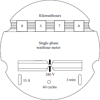
Figure 2.18 shows a single-phase (electromechanical) watthour meter; Figure 2.19 shows its basic parts; Figure 2.20 gives a diagram of a typical motor and magnetic retarding system for a singlephase watthour meter. The magnetic retarding system causes the rotor disk to establish, in combination with the stator, the speed at which the shaft will turn for a given load condition to determine the watthour constant. Figure 2.21a shows a typical socket-mounted two-stator polyphase watthour meter. It is a combination of single-phase watthour meter stators that drive a rotor at a speed proportional to the total power in the circuit.

Single-phase electromechanical watthour meter.
(From General Electric Company, Manual of Watthour Meters, Bulletin GET-1840C.)

Basic parts of a single-phase electromechanical watthour meter.
(From General Electric Company, Manual of Watthour Meters, Bulletin GET-1840C.)
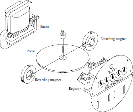
Diagram of a typical motor and magnetic retarding system for a single-phase electromechanical watthour meter.
(From General Electric Company, Manual of Watthour Meters, Bulletin GET-1840C.)
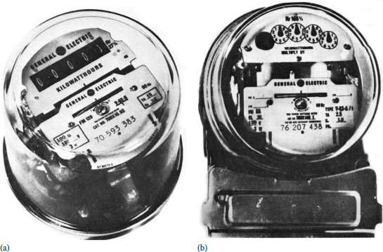
Typical polyphase (electromechanical) watthour meters: (a) self-contained meter (socket-connected cyclometer type). (b) transformer-rated meter (bottom-connected pointer type).
(From General Electric Company, Manual of Watthour Meters, Bulletin GET-1840C.)
The watthour meters used to measure the electric energy passing through various parts of generation, transmission, and distribution systems are required to measure large quantities of electric energy at relatively high voltages. For those applications, transformer-rated meters are developed. They are used in conjunction with standard instrument transformers, that is, current transformers (CTs) and potential transformers (PTs). These transformers reduce the voltage and the current to values that are suitable for low-voltage and low-current meters. Figure 2.21b shows a typical transformer-rated meter. Figure 2.22 shows a single-phase, two-wire watthour electromechanical meter connected to a high-voltage circuit through CTs and PTs.
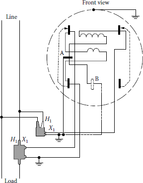
Single-phase, two-wire electromechanical watthour meter connected to a high-voltage circuit through current and potential transformers.
(From General Electric Company, Manual of Watthour Meters, Bulletin GET-1840C.)
A demand meter is basically a watthour meter with a timing element added. The meter functions as an integrator and adds up the kilowatthours of energy used in a certain time interval, for example, 15, 30, or 60 min. Therefore, the demand meter indicates energy per time interval, or average power, which is expressed in kilowatts. Figure 2.23 shows a demand register.
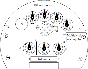
The register of an electromechanical demand meter for large customers.
(From General Electric Company, Manual of Watthour Meters, Bulletin GET-1840C.)
2.7.1 Electronic (or Digital) Meters
Utility companies have started to use new electronic (or digital) meters with programmable demand registers (PDRs) since 1980s. At the first stage of the evolution, the same electromechanical devices used electronic registers. Such electronic register provided a digital display of energy and demand to an electromechanical meter. In the last stage of the evolution, the meters became totally electronic (or solid-state) designed meters.
Such electronic meters have no moving parts. They are built instead around large-scale integrated circuits, other solid-state components, and digital logic. The operation of an electronic meter is very different than the electromechanical meters. The electronic circuitry samples the voltage and current waveforms during each electrical cycle and converts them into digital quantities. Other circuitry then manipulates these values to determine numerous electrical parameters, such as kW, kWh, kvar, kvarh, PF, kVA, rms current, and rms voltage.
A PDR can also measure demand, whereas a traditional register measures only the amount of electricity used in a month. A demand profile shows how much electricity a customer used in a month. Industrial and commercial customers are billed according to their peak demand for the month, as well as their kWh consumption. Utilities have been using supplementary devices with the traditional meters to measure demand. But the PDR measures total kWh used, demand, and cumulative demand by itself.
Here, measuring cumulative demand is a security measure. If the cumulative demand doesn’t equal to the sum of the monthly demands, then someone may have tampered with the meter. It will automatically add the demand reading to the cumulative each time it is reset, so a meter will know if someone reset it since he or she was there last.
The PDR may also be programmed to record the date each time it is reset. The PDR can also be programmed in many other ways. For example, it can alert a customer when he reaches a certain demand level, so that the customer could cut back if he or she wants it.
Today, electronic meters can also measure some or all of the following capabilities:
- Time of use (TOU): The meter keeps up with energy and demand in multiple daily periods.
- Bidirectional: The meter measures (as separate quantities) energy delivered to and received from a customer. (It can be used by a customer who is able to generate electricity and sell to a utility company.)
- Interval data recording: The meter has solid-state memory in which it can record up to several months of interval-by-interval data.
- Remote communications: Its built-in communication capabilities allow the meter to be interrogated remotely via radio, telephone, or other communications media.
- Diagnostics: The meter checks for the proper voltage, currents, and phase angles on the meter conductors.
- Loss compensation: It can be programmed to automatically calculate watt and var losses in transformers and electrical conductors based on defined or tested loss characteristics of the transformers and conductors.
2.7.2 Reading Electric Meters
By reading the register, that is, the revolution counter, the customers’ bills can be determined. There are primarily two different types of registers: (1) conventional dial and (2) cyclometer.
Figure 2.24 shows a conventional dial-type register. To interpret it, read the dials from left to right. (Note that numbers run clockwise on some dials and counterclockwise on others.) The figures above each dial show how many kilowatthours are recorded each time the pointer makes a complete revolution.
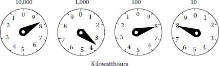
As shown in Figure 2.24, if the pointer is between numbers, read the smaller one. The number 0 stands for 10. If the pointer is pointed directly at a number, look at the dial to the right. If that pointer has not yet passed 0, record the smaller number; if it has passed 0, record the number the pointer is on. For example, in Figure 2.24, the pointer on the first dial is between 8 and 9; therefore read 8. The pointer on the second dial is between 3 and 4; thus read 3. The pointer on the third dial is almost directly on 8, but the dial on the right has not reached 0 so the reading on the third dial is 7. The fourth dial reading is 8. Therefore, the total reading is 8378 kWh. The third dial would be read as 8 after the pointer on the 10-kWh dial reaches 0. This reading is based on a cumulative total, that is, since the meter was last set at 0, 8378 kWh of electricity has been used.
To find the customer’s monthly use, take two readings 1 month apart and subtract the earlier one from the later one. Some electric meters have a constant, or multiplier, indicated on the meter. This type of meter is primarily for high-usage customers.
Figure 2.25 shows a cyclometer-type register. Here, even though the procedure is the same as in the conventional type, the wheels, which indicate numbers directly, replace the dials. Therefore, it makes possible the reading of the meter simply and directly, from left to right.
2.7.3 Instantaneous Load Measurements Using Electromechanical Watthour Meters
The instantaneous kilowatt demand of any customer may be determined by making field observations of the kilowatthour meter serving the customer. However, the instantaneous load measurement should not replace demand meters that record for longer time intervals. The instantaneous demand may be determined by using one of the following equations:
- For a self-contained watthour meter,
- For a transformer-rated meter (where instrument transformers are used with a watthour meter),
where
Di is the instantaneous demand, kW
Kr is the number of meter disk revolutions for a given time period
Kh is the watthour meter constant (given on the register), Wh/rev
T is the time, s
CTR is the current transformer ratio
PTR is the potential transformer ratioSince the kilowatt demand is based on a short-time interval, two or more demand intervals should be measured. The average value of these demands is a good estimate of the given customer’s kilowatt demand during the intervals measured.
Example 2.17
Assume that the load is measured twice with a watthour meter that has a meter constant of 7.2 and the following data are obtained:
First Reading |
Second Reading |
|
|---|---|---|
Revolutions of disk |
32 |
27 |
Time interval for revolutions of disks |
59 |
40 |
Determine the instantaneous demands and the average demand.
Solution
From Equation 2.47, for the first reading,
and for the second reading,
Therefore, the average demand is
Example 2.18
Assume that the data given in Example 2.17 are the results of load measurement with watthour meters and instrument transformers. Suppose that the new meter constant is 1.8 and that the ratios of the CTs and PTs used are 200 and 1, respectively. Determine the instantaneous demands for both readings and the average demand.
Solution
Therefore, from Equation 2.48,
and
Thus the average demand is
Example 2.19
Assume that the load is measured with watthour and varhour meters and instrument transformers and that the following readings are obtained:
Watthour Readings |
Varhour Readings |
|||
|---|---|---|---|---|
First set |
Second set |
First set |
Second set |
|
Revolutions of disk |
20 |
30 |
10 |
20 |
Time interval for revolutions of disks |
50 |
60 |
50 |
60 |
Assume that the new meter constants are 1.2 and that the ratios of the current and potential transformers used are 80 and 20, respectively. Determine the following:
- The instantaneous kilowatt demands
- The average kilowatt demand
- The instantaneous kilovar demands
- The average kilovar demand
- The average kilovoltampere demand
Solution
- The instantaneous kilowatt demands are
and
- The average kilowatt demand is
- The instantaneous kilovar demands are
and
- The average kilovar demand is
- The average kilovoltampere demand is
Problems
- 2.1 Use the data given in Example 2.1 and assume that the feeder has the peak loss of 72 kW at peak load and an annual loss factor of 0.14. Determine the following:
- The daily average load of the feeder
- The average power loss of the feeder
- The total annual energy loss of the feeder
- 2.2 Use the data given in Example 2.1 and the equations given in Section 2.2 and determine the load factor of the feeder.
- 2.3 Use the data given in Example 2.1 and assume that the connected demands for the street lighting load, the residential load, and the commercial load are 100, 2000, and 2000 kW, respectively. Determine the following:
- The DF of the street lighting load
- The DF of the residential load
- The DF of the commercial load
- The DF of the feeder
- 2.4 Using the data given in Table P.2.1 for a typical summer day, repeat Example 2.1 and compare the results.
- 2.5 Use the data given in Problem 2.4 and repeat Problem 2.2.
- 2.6 Use the data given in Problem 2.4 and repeat Problem 2.3.
- 2.7 Use the result of Problem 2.2 and calculate the associated loss factor.
- 2.8 Assume that a load of 100 kW is connected at the Riverside substation of the NL&NP Company. The 15-min weekly maximum demand is given as 75 kW, and the weekly energy consumption is 4200 kWh. Assuming a week is 7 days, find the DF and the 15-min weekly load factor of the substation.
- 2.9 Assume that the total kilovoltampere rating of all DTs connected to a feeder is 3000 kVA. Determine the following:
- If the average core loss of the transformers is 0.50%, what is the total annual core loss energy on this feeder?
- Find the value of the total core loss energy calculated in part (a) at $0.025/kWh.
- 2.10 Use the data given in Example 2.6 and also consider the following added new load. Suppose that several buildings that have electric air-conditioning are converted from gas-fired heating to electric heating. Let the new electric heating load average 200 kW during 6 months of heating (and off-peak) season. Assume that off-peak energy delivered to these primary feeders costs the NL&NP Company 2 cents/kWh and that the capacity cost of the power system remains at $3.00/kW per month.
- Find the new annual load factor on the substation.
- Find the total annual cost to NL&NP to serve this new load.
- Why is it that the hypothetical but illustrative energy cost is smaller in this problem than the one in Example 2.8?
- 2.11 The input to a subtransmission system is 87,600,000 kWh annually. On the peak-load day of the year, the peak is 25,000 kW and the energy input that day is 300,000 kWh. Find the load factors for the year and for the peak-load day.
Typical Summer-Day Load, in kW
Time
Street Lighting
Residential
Commercial
12 AM
100
250
300
1
100
250
300
2
100
250
300
3
100
250
300
4
100
250
300
5
100
250
300
6
100
250
300
7
350
300
8
450
400
9
550
600
10
550
1100
11
550
1100
12 noon
600
1100
1
600
1100
2
600
1300
3
600
1300
4
600
1300
5
650
1300
6
750
900
7
900
500
8
100
1100
500
9
100
1100
500
10
100
900
300
11
100
700
300
12 PM
100
350
300
- 2.12 The electric energy consumption of a residential customer has averaged 1150 kWh/month as follows, starting in January: 1400, 900, 1300, 1200, 800, 700, 1000, 1500, 700, 1500, 1400, and 1400 kWh. The customer is considering purchasing equipment for a hobby shop that he has in his basement. The equipment will consume about 200 kWh each month. Estimate the additional annual electric energy cost for operation of the equipment. Use the electrical rate schedule given in the following table.
Residential
Rate: (net) per month per meter
Energy Charge
For the first 25 kWh
6.00 ȼ/kWh
For the next 125 kWh
3.2 ȼ/kWh
For the next 850 kWh
2.00 ȼ/kWh
All in excess of 1000 kWh
1.00 ȼ/kWh
Minimum: $1.50 per month
Commercial
A rate available for general, commercial, and miscellaneous power uses where consumption of energy does not exceed 10,000 kWh in any month during any calendar year.
Rate: (net) per month per meter
Energy Charge
For the first 25 kWh
6.0 ȼ/kWh
For the next 375 kWh
4.0 ȼ/kWh
For the next 3600 kWh
3.0 ȼ/kWh
All in excess of 4000 kWh
1.5 ȼ/kWh
Minimum: $1.50 per month
General power
A rate available for service supplied to any commercial or industrial customer whose consumption in any month during the calendar year exceeds 10,000 kWh. A customer who exceeds 10,000 kWh per month in any 1 month may elect to receive power under this rate.
A customer who exceeds 10,000 kWh in any 3 months or who exceeds 12,000 kWh in any 1 month during a calendar year shall be required to receive power under this rate at the option of the supplier.
A customer who elects at his own option to receive power under this rate may not return to the commercial service rate except at the option of the supplier.
Rate: (net) per month per meter kW is rate of flow. 1 kW for l h is 1 kWh.
Demand charge
For the first 30 kW of maximum demand per month
$2.50/kW
For all maximum demand per month in excess of 30 kW
$1.25/kW
Energy Charge
For the first 100 kWh per kW of maximum demand per month
2.00 ȼ/kWh
For the next 200 kWh per kW of maximum demand per month
1.2 ȼ/kWh
All in excess of 300 kWh per kW of maximum demand per month
0.5 ȼ/kWh
Minimum charge: The minimum monthly bill shall be the demand charge for the month. Determination of maximum demand: The maximum demand shall be either the highest integrated kW load during any 30 min period occurring during the billing month for which the determination is made or 75% of the highest maximum demand that has occurred in the preceding month, whichever is greater.
Water heating: 1.00/kWh with a minimum monthly charge of $1.00.
- 2.13 The Zubits International Company, located in Ghost Town, consumed 16,000 kWh of electric energy for Zubit production this month. The company’s monthly average energy consumption is also 16,000 kWh due to some unknown reasons. It has a 30 min monthly maximum demand of 200 kW and a connected demand of 580 kW. Use the electrical rate schedule given in Problem 2.12.
- Find the Zubits International’s total monthly electrical bill for this month.
- Find its 30 min monthly load factor.
- Find its DF.
- The company’s newly hired plant engineer, who recently completed a load management course at Ghost University, suggested that, by shifting the hours of a certain production from the peak-load hours to off-peak hours, the maximum monthly demand can be reduced to 140 kW at a cost of $50/month. Do you agree that this will save money? How much?
- 2.14 Repeat Example 2.12, assuming that there are eight houses connected on each DT and that there are a total of 120 DTs and 960 residences supplied by the primary feeder.
- 2.15 Repeat Example 2.15, assuming that the 30 min monthly maximum demands of customers A and B are 27 and 42 kW, respectively. The new monthly energy consumptions by customers A and B are 8000 and 9000 kWh, respectively. The new lagging load PFs of A and B are 0.90 and 0.70, respectively.
- 2.16 A customer transformer has 12 residential customers connected to it. Connected load is 20 kW per house, DF is 0.6, and diversity factor is 1.15. Find the diversified demand of the group of 12 houses on the transformer.
- 2.17 A distribution substation is supplied by total annual energy of 100,000 MWh. If its annual average load factor is 0.6, determine the following:
- The annual average power demand
- The maximum monthly demand
- 2.18 Suppose that one of the transformers of a substation supplies four primary feeders. Among the four feeders, the diversity factor is 1.25 for both real power (P) and reactive power (Q). The 30 min annual demands of per feeder with their PFs at the time of annual peak load are shown as follows:
Feeder
Demand (kW)
PF
1
900
0.85
2
1000
0.9
3
2100
0.95
4
2000
0.9
- Find the 30 min annual maximum demand on the substation transformer in kW and in kVA.
- Find the load diversity in kW.
- Select a suitable substation transformer size if zero load growth is expected and company policy permits as much as 25% short-time overloads on the transformer. Among the standard three-phase transformer sizes available are the following:
- 2500/3125 kVA self-cooled/forced-air-cooled
- 3750/4687 kVA self-cooled/forced-air-cooled
- 50006250 kVA self-cooled/forced-air-cooled
- 7500/9375 kVA self-cooled/forced-air-cooled
- Now assume that the substation load will increase at a constant percentage rate per year and will double in 10 years. If 7500/9375 kVA-rated transformer is installed, in how many years will it be loaded to its fans-on rating?
- 2.19 Suppose that a primary feeder is supplying power to a variable load. Every day and all year long, the load has a daily constant peak value of 50 MW between 7 PM and 7 AM and a daily constant off-peak value of 5 MW between 7 AM and 7 PM. Derive the necessary equations and calculate the following:
- The load factor of the feeder
- The factor of the feeder
- 2.20 A typical DT serves four residential loads, that is, houses, through six SDs and two spans of SL. There are a total of 200 DTs and 800 residences supplied by this primary feeder. Use Figure 2.13 and Table 2.2 and assume that a typical residence has a clothes dryer, a range, a refrigerator, and some lighting and miscellaneous appliances. Determine the following:
- The 30 min maximum diversified demand on the transformer
- The 30 min maximum diversified demand on the entire feeder
- Use the typical hourly variation factors given in Table 2.2 and calculate the small portion of the daily demand curve on the DT, that is, the total hourly diversified demands at 6 AM, 12 noon, and 7 PM, on the DT, in kilowatts
- 2.21 Repeat Example 2.15, assuming that the monthly demand charge is $15/kW and that the monthly energy charges are 12 cents/kWh for the first 1000 kWh, 10 cents/kWh for the next 3000 kWh, and 8 cents/kWh for all kWh in excess of 4000. The 30 min maximum diversified demands for customers A and B are 40 kW each. The PFs for customers A and B are 0.95 lagging and 0.50 lagging, respectively.
- 2.22 Consider the MATLAB demand forecasting computer program given in Table 2.3. Assume that the peak MW July demands for the last 8 years have been the following: 3094, 2938, 2714, 3567, 4027, 3591, 4579, and 4436. Use the given MATLAB program as a curve-fitting technique and determine the following:
- The average rate of growth of the demand
- The ideal data based on rate of growth for the past 8 years to give the correct future demand forecast
- The forecasted future demands for the next 10 years
- 2.23 The annual peak load of the feeder is 3000 kWh. Total copper loss at peak load is 300 kW. If the total annual energy supplied to the sending end of the feeder is 9000 MWh, determine the following:
- The annual loss factor for an urban area
- The annual loss factor for a rural area
- The total amount of energy lost due to copper losses per year in part (a) and its value at $0.06/kWh
- The total amount of energy lost due to copper losses per year in part (b) and its value at $0.06/kWh.
References
1. ASA: American Standard Definitions of Electric Terms, Group 35, Generation, Transmission and Distribution, ASA C42.35, Alexandra, VA, 1957.
2. Westinghouse Electric Corporation: Electric Utility Engineering Reference Book-Distribution Systems, Vol. 3, Westinghouse Electric Corporation, East Pittsburgh, PA, 1965.
3. Sarikas, R. H. and H. B. Thacker: Distribution system load characteristics and Their use in planning and Design, AIEE Trans., 31(pt. III), August 1957, 564–573.
4. Seelye, H. P.: Electrical Distribution Engineering, McGraw-Hill, New York, 1930.
5. Buller, F. H. and C. A. Woodrow: Load factor-equivalent hour values compared, Electr. World, 92(2), July 14, 1928, 59–60.
6. General Electric Company: Manual of Watthour Meters, Bulletin GET-1840C, Schenectady, New York.
7. Arvidson, C. E.: Diversified demand method of estimating residential distribution transformer loads, Edison Electr. Inst. Bull., 8, October 1940, 469–479.
8. Box, G. P. and G. M. Jenkins: Time Series Analysis, Forecasting and Control, Holden-Day, San Francisco, CA, 1976.
9. ABB Power T & D Company: Introduction to Integrated Resource T & D Planning, Cory, NC, 1994.
10. Willis, H. L.: Spatial Electric Load Forecasting, Marcel Dekker, New York, 1996.
11. Gönen, T. and J. C. Thompson: A new stochastic load forecasting model to predict load growth on radial feeders, Int. J. Comput. Math. Electr. Electron. Eng. (COMPEL), 3(1), 1984, 35–46.
13. Thompson, J. C. and T. Gönen: A developmental system simulation of growing electrical energy demand, IEEE Mediterranean Electrotechnical Conference (MELECON 83), Rome, Italy, May 24–26, 1983.
14. Thompson, J. C. and T. Gönen: Simulation of load growth developmental system models for comparison with field data on radial networks, Proceedings of the 1982 Modeling and Simulation Conference, University of Pittsburgh, Pittsburgh, PA, April 22–23, 1982, Vol. 13, pt. 4, pp. 1549–1554.
15. Gönen, T. and A. Saidian: Electrical Load Forecasting, Proceedings of the 1981 Modeling and Simulation Conference, University of Pittsburgh, Pittsburgh, PA, April 30–May 1, 1981.
16. Ramirez-Rosado, I. J. and T. Gönen: Economical and energetic benefits derived from selected demandside management actions in the electric power distribution, International Conference on Modeling, Identification, and Control, Zurich, Switzerland, February 1998.
17. Gellings, C. W.: Demand Forecasting for Electric Utilities, The Fairmont Press, Lilburn, GA, 1992.
*It is calculated from P(0.85/PF). However, if the PF is greater than 0.85, then still the actual amount of P is used, rather than the resultant kW.