Chapter 7

Voltage-Drop and Power-Loss Calculations

Any man may make a mistake; none but a fool will stick to it.

M.T. Cicero, 51 B.C.

Time is the wisest counselor.

Pericles, 450 B.C.

When others agree wth me, I wonder what is wrong!

Author Unknown

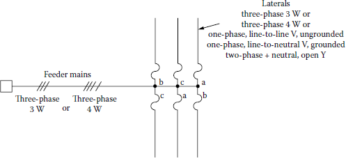
7.1 Three-Phase Balanced Primary Lines

As discussed in Chapter 5, a utility company strives to achieve a well-balanced distribution system in order to improve system voltage regulation by means of equally loading each phase. Figure 7.1 shows a primary system with either a three-phase three-wire or a three-phase four-wire main. The laterals can be either (1) three-phase three-wire, (2) three-phase four-wire, (3) single phase with line-to-line voltage, ungrounded, (4) single phase with line-to-neutral voltage, grounded, or (5) two-phase plus neutral, open wye.

7.2 Non-Three-Phase Primary Lines

Usually there are many laterals on a primary feeder that are not necessarily in three phase, for example, single phase, which causes the voltage drop and power loss due to load current not only in the phase conductor but also in the return path.

7.2.1 Single-Phase Two-Wire Laterals with Ungrounded Neutral

Assume that an overloaded single-phase lateral is to be changed to an equivalent three-phase three-wire and balanced lateral, holding the load constant. Since the power input to the lateral is the same as before,

$\begin{array}{cc}{S}_{1\varphi }=S_{3\varphi }\hfill & (7.1)\hfill \end{array}$

(From Gonen’s book Electric Power Distribution System Engineering, Figure 7.1 on page 324.) where the subscripts 1ϕ and 3ϕ refer to the single-phase and three-phase circuits, respectively. Equation 7.1 can be rewritten as

$\begin{array}{cc}(\sqrt{3}\times V_s)I_{1\varphi }=3V_s{I}_{3\varphi }\hfill & (7.2)\hfill \end{array}$

where Vs is the line-to-neutral voltage. Therefore, from Equation 7.2,

$\begin{array}{cc}{I}_{1\varphi }=\sqrt{3}\times I_{3\varphi }\hfill & (7.3)\hfill \end{array}$

which means that the current in the single-phase lateral is 1.73 times larger than the one in the equivalent three-phase lateral. The voltage drop in the three-phase lateral can be expressed as

$\begin{array}{cc}{\text{VD}}_{3\varphi }=I_{3\varphi }(R\cos \theta +X\sin \theta )\hfill & (7.4)\hfill \end{array}$

and in the single-phase lateral as

$\begin{array}{cc}{\text{VD}}_{1\varphi }=I_{1\varphi }(K_{R}R\cos \theta +K_{X}X\sin \theta )\hfill & (7.5)\hfill \end{array}$

where

KR and KX are conversion constants of R and X and are used to convert them from their three-phase values to the equivalent single-phase values

KR = 2.0

KX = 2.0 when underground (UG) cable is used

KX ≅ 2.0 when overhead line is used, with approximately a ±10% accuracy

Therefore, Equation 7.5 can be rewritten as

$\begin{array}{cc}{\text{VD}}_{1\varphi }=I_{1\varphi }(2R\cos \theta +2X\sin \theta )\hfill & (7.6)\hfill \end{array}$

or substituting Equation 7.3 into Equation 7.6,

$\begin{array}{cc}{\text{VD}}_{1\varphi }=2\sqrt{3}\times I_{3\varphi }(R\cos \theta +X\sin \theta )\hfill & (7.7)\hfill \end{array}$

By dividing Equation 7.7 by Equation 7.4 side by side,

$\begin{array}{cc}\frac{{\text{VD}}_{1\varphi }}{{\text{VD}}_{3\varphi }}=2\sqrt{3}\hfill & (7.8)\hfill \end{array}$

which means that the voltage drop in the single-phase ungrounded lateral is approximately 3.46 times larger than the one in the equivalent three-phase lateral. Since base voltages for the single-phase and three-phase laterals are

$\begin{array}{cc}{V}_{B(1\varphi )}=\sqrt{3}\times V_{s,L-N}\hfill & (7.9)\hfill \end{array}$

and

$\begin{array}{cc}{V}_{B(3\varphi )}=V_{s,L-N}\hfill & (7.10)\hfill \end{array}$

Equation 7.8 can be expressed in per units as

$\begin{array}{cc}\frac{{\text{VD}}_{\text{pu,1}\varphi }}{{\text{VD}}_{\text{pu}.3\varphi }}=2.0\hfill & (7.11)\hfill \end{array}$

which means that the per unit voltage drop in the single-phase ungrounded lateral is two times larger than the one in the equivalent three-phase lateral. For example, if the per unit voltage drop in the single-phase lateral is 0.10, it would be 0.05 in the equivalent three-phase lateral.

The power losses due to the load currents in the conductors of the single-phase lateral and the equivalent three-phase lateral are

$\begin{array}{cc}{P}_{LS,1\varphi }=2\times I_{1\varphi }^{2}R\hfill & (7.12)\hfill \end{array}$

and

$\begin{array}{cc}{P}_{LS,3\varphi }=3\times I_{3\varphi }^{2}R\hfill & (7.13)\hfill \end{array}$

respectively. Substituting Equation 7.3 into Equation 7.12,

$\begin{array}{cc}{P}_{LS,1\varphi }=2{\left(\sqrt{3}\times I_{3\varphi }\right)}^{2}R\hfill & (7.14)\hfill \end{array}$

and dividing the resultant Equation 7.14 by Equation 7.13 side by side,

$\begin{array}{cc}\frac{P_{LS,1\varphi }}{P_{LS,3\varphi }}=2.0\hfill & (7.15)\hfill \end{array}$

which means that the power loss due to the load currents in the conductors of the single-phase lateral is two times larger than the one in the equivalent three-phase lateral.

Therefore, one can conclude that by changing a single-phase lateral to an equivalent three-phase lateral, both the per unit voltage drop and the power loss due to copper losses in the primary line are approximately halved.

7.2.2 Single-Phase Two-Wire Ungrounded Laterals

In general, this system is presently not used due to the following disadvantages. There is no earth current in this system. It can be compared to a three-phase four-wire balanced lateral in the following manner. Since the power input to the lateral is the same as before,

$\begin{array}{cc}{S}_{1\varphi }=S_{3\varphi }\hfill & (7.16)\hfill \end{array}$

or

$\begin{array}{cc}{V}_s\times I_{1\varphi }=3\times V_s\times I_{3\varphi }\hfill & (7.17)\hfill \end{array}$

from which

$\begin{array}{cc}{I}_{1\varphi }=3\times I_{3\varphi }\hfill & (7.18)\hfill \end{array}$

The voltage drop in the three-phase lateral can be expressed as

$\begin{array}{cc}{\text{VD}}_{3\varphi }=I_{3\varphi }(R\cos \theta +X\sin \theta )\hfill & (7.19)\hfill \end{array}$

and in the single-phase lateral as

$\begin{array}{cc}{\text{VD}}_{1\varphi }=I_{1\varphi }(K_{R}R\cos \theta +K_{X}X\sin \theta )\hfill & (7.20)\hfill \end{array}$

where

KR = 2.0 when a full-capacity neutral is used, that is, if the wire size used for neutral conductor is the same as the size of the phase wire

KR > 2.0 when a reduced-capacity neutral is used

KX ≅ 2.0 when overhead line is used

Therefore, if KR = 2.0 and KX = 2.0, Equation 7.20 can be rewritten as

$\begin{array}{cc}{\text{VD}}_{1\varphi }=I_{1\varphi }(2R\cos \theta +2X\sin \theta )\hfill & (7.21)\hfill \end{array}$

or substituting Equation 7.18 into Equation 7.21,

$\begin{array}{cc}{\text{VD}}_{1\varphi }=6\times I_{3\varphi }(R\cos \theta +X\sin \theta )\hfill & (7.22)\hfill \end{array}$

Dividing Equation 7.22 by Equation 7.19 side by side,

$\begin{array}{cc}\frac{{\text{VD}}_{1\varphi }}{{\text{VD}}_{3\varphi }}=6.0\hfill & (7.23\text{a})\hfill \end{array}$

or

$\begin{array}{cc}\frac{{\text{VD}}_{\text{pu,1}\varphi }}{{\text{VD}}_{\text{pu,1}\varphi }}=2\sqrt{3}=3.46\hfill & (7.23\text{b})\hfill \end{array}$

which means that the voltage drop in the single-phase two-wire ungrounded lateral with full-capacity neutral is six times larger than the one in the equivalent three-phase four-wire balanced lateral.

The power losses due to the load currents in the conductors of the single-phase two-wire unigrounded lateral with full-capacity neutral and the equivalent three-phase four-wire balanced lateral are

$\begin{array}{cc}{P}_{\text{LS},1\varphi }=I_{1\varphi }^2(2R)\hfill & (7.24)\hfill \end{array}$

and

$\begin{array}{cc}{P}_{\text{LS},3\varphi }=3\times I_{3\varphi }^{2}R\hfill & (7.25)\hfill \end{array}$

respectively. Substituting Equation 7.18 into Equation 7.24,

$\begin{array}{cc}{P}_{\text{LS},1\varphi }={(3\times I_{3\varphi })}^2(2R)\hfill & (7.26)\hfill \end{array}$

and dividing Equation 7.26 by Equation 7.25 side by side,

$\begin{array}{cc}\frac{P_{\text{LS},1\varphi }}{P_{\text{LS},3\varphi }}=6.0\hfill & (7.27)\hfill \end{array}$

Therefore, the power loss due to load currents in the conductors of the single-phase two-wire unigrounded lateral with full-capacity neutral is six times larger than the one in the equivalent three-phase four-wire lateral.

7.2.3 Single-Phase Two-Wire Laterals with Multigrounded Common Neutrals

Figure 7.2 shows a single-phase two-wire lateral with multigrounded common neutral. As shown in the figure, the neutral wire is connected in parallel (i.e., multigrounded) with the ground wire at various places through ground electrodes in order to reduce the current in the neutral. Ia is the current in the phase conductor, Iw is the return current in the neutral wire, and Id is the return current in Carson’s equivalent ground conductor. According to Morrison [1], the return current in the neutral wire is

$\begin{array}{cc}{I}_n={\zeta }_1{I}_a\text{where}{\zeta }_1=0.25-0.33\hfill & (7.28)\hfill \end{array}$

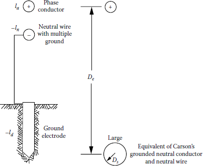
and it is almost independent of the size of the neutral conductor.

In Figure 7.2, the constant KR is less than 2.0 and the constant KX is more or less equal to 2.0 because of conflictingly large Dm (i.e., mutual geometric mean distance or geometric mean radius) of Carson’s equivalent ground (neutral) conductor. Therefore, Morrison’s data [1] (probably empirical) indicate that

$\begin{array}{cc}{\text{VD}}_{\text{pu,1}\varphi }={\zeta }_2\times {\text{VD}}_{\text{pu,3}\varphi }\text{where }{\zeta }_2=3.8-4.2\hfill & (7.29)\hfill \end{array}$

and

$\begin{array}{cc}{\text{P}}_{\text{LS,1}\varphi }={\zeta }_3\times {\text{P}}_{\text{LS,3}\varphi }\text{where}{\zeta }_3=3.5-3.75\hfill & (7.30)\hfill \end{array}$

Therefore, assuming that the data from Morrison [1] are accurate,

$K_R<2.0\text{and}{K}_X<2.0$

the per unit voltage drops and the power losses due to load currents can be approximated as

$\begin{array}{cc}{\text{VD}}_{\text{pu,1}\varphi }\cong 4.0\times {\text{VD}}_{\text{pu,3}\varphi }\hfill & (7.31)\hfill \end{array}$

and

$\begin{array}{cc}{\text{P}}_{\text{LS}}{{}_{,}}_{1\varphi }\cong 3.6\times {\text{P}}_{\text{LS,3}\varphi }\hfill & (7.32)\hfill \end{array}$

for the illustrative problems.

7.2.4 Two-Phase Plus Neutral (Open-Wye) Laterals

Figure 7.3 shows an open-wye-connected lateral with two phase and neutral. The neutral conductor can be unigrounded or multigrounded, but because of disadvantages, the unigrounded neutral is generally not used. If the neutral is unigrounded, all neutral current is in the neutral conductor itself. Theoretically, it can be expressed that

$\begin{array}{cc}\text{V=ZI}\hfill & (7.33)\hfill \end{array}$

where

$\begin{array}{cc}{\overline{\text{V}}}_a={\overline{Z}}_a{\overline{I}}_a\hfill & (7.34)\hfill \end{array}$

$\begin{array}{cc}{\overline{\text{V}}}_b={\overline{Z}}_b{\overline{I}}_b\hfill & (7.35)\hfill \end{array}$

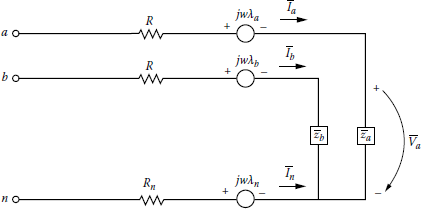
It is correct for equal load division between the two phases.

Assuming equal load division among phases, the two-phase plus neutral lateral can be compared to an equivalent three-phase lateral, holding the total kilovoltampere load constant. Therefore,

$\begin{array}{cc}{S}_{2\varphi }=S_{3\varphi }\hfill & (7.36)\hfill \end{array}$

or

$\begin{array}{cc}2V_5{I}_{2\varphi }=3V_5{I}_{3\varphi }\hfill & (7.37)\hfill \end{array}$

from which

$\begin{array}{cc}{I}_{2\varphi }=\frac{3}{2}{I}_{3\varphi }\hfill & (7.38)\hfill \end{array}$

The voltage-drop analysis can be performed depending upon whether the neutral is unigrounded or multigrounded. If the neutral is unigrounded and the neutral conductor impedance (Zn) is zero, the voltage drop in each phase is

$\begin{array}{cc}{\text{VD}}_{2\varphi }=I_{2\varphi }\left(K_{R}R\cos \theta +K_{X}X\sin \theta \right)\hfill & (7.39)\hfill \end{array}$

where

KR = 1.0

KX = 1.0

Therefore,

$\begin{array}{cc}{\text{VD}}_{2\varphi }=I_{2\varphi }\left(R\cos \theta +X\sin \theta \right)\hfill & (7.40)\hfill \end{array}$

or substituting Equation 7.38 into Equation 7.40,

$\begin{array}{cc}{\text{VD}}_{2\varphi }=\frac{3}{2}{I}_{3\varphi }\left(R\cos \theta +X\sin \theta \right)\hfill & (7.41)\hfill \end{array}$

Dividing Equation 7.41 by Equation 7.19, side by side,

$\begin{array}{cc}\frac{{\text{VD}}_{2\varphi }}{{\text{VD}}_{3\varphi }}=\frac{3}{2}\hfill & (7.42)\hfill \end{array}$

However, if the neutral is unigrounded and the neutral conductor impedance (Zn) is larger than zero,

$\begin{array}{cc}\frac{{\text{VD}}_{2\varphi }}{{\text{VD}}_{3\varphi }}>\frac{3}{2}\hfill & (7.43)\hfill \end{array}$

Therefore, in this case, some unbalanced voltages are inherent.

However, if the neutral is multigrounded and Zn > 0, the data from Morrison [1] indicate that the per unit voltage drop in each phase is

$\begin{array}{cc}{\text{VD}}_{\text{pu,2}\varphi }=2.0\times {\text{VD}}_{\text{pu,3}\varphi }\hfill & (7.44)\hfill \end{array}$

when a full-capacity neutral is used and

$\begin{array}{cc}{\text{VD}}_{\text{pu,2}\varphi }=2.1\times {\text{VD}}_{\text{pu,3}\varphi }\hfill & (7.45)\hfill \end{array}$

when a reduced-capacity neutral (i.e., when the neutral conductor employed is one or two sizes smaller than the phase conductors) is used.

The power loss analysis also depends upon whether the neutral is unigrounded or multigrounded. If the neutral is unigrounded, the power loss is

$\begin{array}{cc}{P}_{\text{LS},2\varphi }=I_{2\varphi }^2\left(K_{R}R\right)\hfill & (7.46)\hfill \end{array}$

where

KR = 3.0 when a full-capacity neutral is used

KR > 3.0 when a reduced-capacity neutral is used

Therefore, if KR = 3.0,

$\begin{array}{cc}\frac{P_{\text{LS},2\varphi }}{P_{\text{LS},3\varphi }}=\frac{3I_{2\varphi }^{2}R}{3I_{3\varphi }^{2}R}\hfill & (7.47)\hfill \end{array}$

or

$\begin{array}{cc}\frac{P_{\text{LS},2\varphi }}{P_{\text{LS},3\varphi }}=2.25\hfill & (7.48)\hfill \end{array}$

On the other hand, if the neutral is multigrounded,

$\begin{array}{cc}\frac{P_{\text{LS},2\varphi }}{P_{\text{LS},3\varphi }}<2.25\hfill & (7.49)\hfill \end{array}$

Based on the data from Morrison [1], the approximate value of this ratio is

$\begin{array}{cc}\frac{P_{\text{LS,}2\varphi }}{P_{\text{LS},3\varphi }}\cong 1.64\hfill & (7.50)\hfill \end{array}$

which means that the power loss due to load currents in the conductors of the two-phase three-wire lateral with multigrounded neutral is approximately 1.64 times larger than the one in the equivalent three-phase lateral.

Example 7.1

Assume that a uniformly distributed area is served by a three-phase four-wire multigrounded 6-mile-long main located in the middle of the service area. There are six laterals on each side of the main. Each lateral is 1 mile apart with respect to each other, and the first lateral is located on the main 1 mile away from the substation so that the total three-phase load on the main is 6000 kVA. Each lateral is 10 mi long and is made up of #6 AWG copper conductors and serving a uniformly distributed peak load of 500 kVA, at 7.2/12.47 kV. The K constant of a #6 AWG copper conductor is 0.0016/kVA-mi. Determine the following:

1. The maximum voltage drop to the end of each lateral, if the lateral is a three-phase lateral with multigrounded common neutrals
2. The maximum voltage drop to the end of each lateral, if the lateral is a two-phase plus full-capacity multigrounded neutral (open-wye) lateral
3. The maximum voltage drop to the end of each lateral, if the lateral is a single-phase two-wire lateral with multigrounded common neutrals

Solution

1. For the three-phase four-wire lateral with multigrounded common neutrals,

   $\begin{array}{lll}\%{\text{VD}}_{3\varphi }\hfill & =\hfill & \frac{1}{2}\times K\times S\hfill \\ \hfill & =\hfill & \left(\frac{10\text{mi}}{2}\right)\left(0.0016\frac{\%\text{VD}}{\text{kVA–mi}}\right)\left(500\text{kVA}\right)=4\hfill \end{array}$

2. For the two-phase plus full-capacity multigrounded neutral (open-wye) lateral, according to the results of Morrison,

   $\begin{array}{lll}\%{\text{VD}}_{2\varphi }\hfill & =\hfill & 2\left(\%{\text{VD}}_{3\varphi }\right)\hfill \\ \hfill & =\hfill & 2(4\%)=8\hfill \end{array}$

3. For the single-phase two-wire lateral with multigrounded common neutrals, according to the results of Morrison,

   $\begin{array}{lll}\%{\text{VD}}_{1\varphi }\hfill & =\hfill & 4\left(\%{\text{VD}}_{3\varphi }\right)\hfill \\ \hfill & =\hfill & 4(4\%)=16\hfill \end{array}$

Example 7.2

A three-phase express feeder has an impedance of 6 + j20 ohms per phase. At the load end, the line-to-line voltage is 13.8 kV, and the total three-phase power is 1200 kW at a lagging power factor of 0.8. By using the line-to-neutral method, determine the following:

1. The line-to-line voltage at the sending end of the feeder (i.e., at the substation low-voltage bus)
2. The power factor at the sending end
3. The copper loss (i.e., the transmission loss) of the feeder
4. The power at the sending end in kW Solution

Solution

Since in an express feeder, the line current is the same at the beginning or at the end of the line,

$\begin{array}{lll}{I}_L=I_S=I_R\hfill & =\hfill & \frac{P_{R(3\varphi )}}{\sqrt{3}{V}_{R(L-L)}\cos \theta }\hfill \\ \hfill & =\hfill & \frac{1,200\text{kW}}{\sqrt{3}(13.8\text{kV})0.8}=62.75\text{A}\hfill \end{array}$

and

$\begin{array}{lll}{V}_{R(L-N)}\hfill & =\hfill & \frac{V_{R(L-L)}}{\sqrt{3}}\hfill \\ \hfill & =\hfill & \frac{13,800\text{V}}{\sqrt{3}}=7,976.4\text{V}\text{.}\hfill \end{array}$

using this as the reference voltage, the sending-end voltage is found from

${\overline{V}}_{S(L-N)}={\overline{V}}_{R(L-N)}+{\overline{I}}_L{\overline{Z}}_L$

where

${\overline{V}}_{R(L-N)}=7,976.9\angle 0^{\circ }\text{V}$

$\begin{array}{lll}{\overline{I}}_L={\overline{I}}_S={\overline{I}}_R\hfill & =\hfill & I_L\left(\cos {\theta }_R-\sin {\theta }_R\right)\hfill \\ \hfill & =\hfill & 62.83\left(0.8-j0.6\right)=62.83\angle -{36.87}^{\circ }\text{A}\hfill \end{array}$

${\overline{Z}}_L=6+j20=20.88\angle {73.3}^{\circ }\text{Ω}$

1. $\begin{array}{lll}{\overline{V}}_{s(L-N)}\hfill & =\hfill & 7,976.9\angle 0^{\circ }+\left(62.83\angle -{36.87}^{\circ }\right)\left(20.88\angle {73.7}^{\circ }\right)\hfill \\ \hfill & =\hfill & 9,065.95\angle {4.93}^{\circ }\text{V}\hfill \end{array}$

   and

   $\begin{array}{lll}{\overline{V}}_{s(L-L)}\hfill & =\hfill & \sqrt{3}{\overline{V}}_{s(L-N)}\hfill \\ \hfill & =\hfill & \sqrt{3}\left(9,065.95\right)\angle {4.93}^{\circ }+{30}^{\circ }\hfill \\ \hfill & =\hfill & 15,684.09\angle {34.93}^{\circ }\text{V}\hfill \end{array}$

2. ${\theta }_S=\left|{\theta }_{{\overline{V}}_{S(L-N)}}\right|-\left|{\theta }_{{\overline{I}}_S}\right|={4.9}^{\circ }-\left|-{36.87}^{\circ }\right|={41.8}^{\circ }\text{and}\text{cos}{\theta }_S=0.745\text{lagging}$
3. $\begin{array}{lll}{P}_{\text{loss(3}\varphi \text{)}}\hfill & =\hfill & 3I_L^{2}R=3{(62.83)}^2\times 6\hfill \\ \hfill & =\hfill & 71,056.96\text{W}\cong 71.057\text{kW}\hfill \end{array}$
4. $\begin{array}{lll}{P}_{\text{S(3}\varphi \text{)}}\hfill & =\hfill & P_{R(3\varphi )}+P_{\text{loss(3}\varphi \text{)}}\hfill \\ \hfill & =\hfill & 1,200+71.057=1,271.057\text{kW}\hfill \end{array}$

   or

   $\begin{array}{lll}{P}_{S(3\varphi )}\hfill & =\hfill & \sqrt{3}{V}_{S(L-L)}{I}_S\cos \theta s\hfill \\ \hfill & =\hfill & \sqrt{3}(15,684.09)(62.83)0.745\cong 1,270.073\text{kW}\hfill \end{array}$

Example 7.3

Repeat Example 7.2 by using the single-phase equivalent method.

Solution

Here, the single-phase equivalent current is found from

$\begin{array}{lll}{I}_{eq(1\varphi )}\hfill & =\hfill & \frac{P_{3\varphi }}{V_{R(L-L)}\cos \theta }\hfill \\ \hfill & =\hfill & \frac{1200\text{kW}}{(13.8\text{kV})(0.8)}=108.7\text{A}\hfill \end{array}$

where

$I_{eq(1\varphi )}=\sqrt{3}{I}_{3\varphi }$

or

$\begin{array}{lll}{I}_{3\varphi }=I_L\hfill & =\hfill & \frac{I_{eq(1\varphi )}}{\sqrt{3}}\hfill \\ \hfill & =\hfill & \frac{108.7\text{A}}{\sqrt{3}}=62.8\text{A}\hfill \end{array}$

1. $\begin{array}{ccc}{\overline{V}}_{s(L-L)}\hfill & =\hfill & {\overline{V}}_{R(L-L)}+{\overline{I}}_{eq(1\varphi )}{\overline{Z}}_L\hfill \\ \hfill & =\hfill & 13,800\angle 0^{\circ }+\left(108.7\angle -{36.9}^{\circ }\right)\left(20.88\angle {73.3}^{\circ }\right)\hfill \\ \hfill & =\hfill & 15,684.76\angle {4.93}^{\circ }+{30}^{\circ }\text{V}\hfill \end{array}$
2. ${\theta }_S={\theta }_{\overline{V}S(L-N)}-{\theta }_{{\overline{I}}_S}={41.8}^{\circ }\text{so}\text{that}\text{cos}{\theta }_{\text{S}}=0.745\text{lagging}$
3. $\begin{array}{lll}{P}_{\text{loss(3}\varphi \text{)}}\hfill & =\hfill & I_{eq(1\varphi )}^{2}R\hfill \\ \hfill & =\hfill & {108.7}^2\times 6=70.89\text{kW}\hfill \end{array}$
4. $\begin{array}{lll}{P}_{\text{S(3}\varphi \text{)}}\hfill & =\hfill & P_{R(3\varphi )}+P_{\text{loss}}{}_{(3\varphi )}\hfill \\ \hfill & =\hfill & 1,200+70.89=1,270.89\text{kW}\hfill \end{array}$

7.3 Four-Wire Multigrounded Common Neutral Distribution System

Figure 7.4 shows a typical four-wire multigrounded common neutral distribution system. Because of the economic and operating advantages, this system is used extensively. The assorted secondaries can be, for example, either (1) 120/240 V single-phase three wire, (2) 120/240 V three-phase four wire connected in delta, (3) 120/240 V three-phase four-wire connected in open delta, or (4) 120/208 V three-phase four wire connected in grounded wye. Where primary and secondary systems are both existent, the same conductor is used as the common neutral for both systems. The neutral is grounded at each distribution transformer, at various places where no transformers are connected and to water pipes or driven ground electrodes at each user’s service entrance. The secondary neutral is also grounded at the distribution transformer and the service drops (SDs).

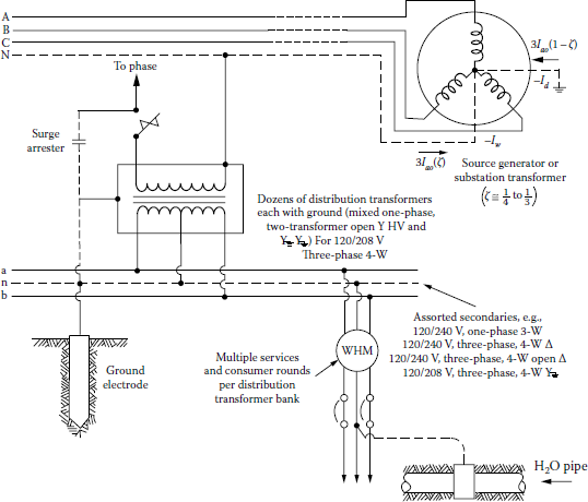
Typical values of the resistances of the ground electrodes are 5, 10, or 15 Ω. Under no circumstances should they be larger than 25 Ω. Usually, a typical metal water pipe system has a resistance value of less than 3 Ω. A part of the unbalanced, or zero sequence, load current flows in the neutral wire, and the remaining part flows in the ground and/or the water system. Usually the same conductor size is used for both phase and neutral conductors.

Example 7.4

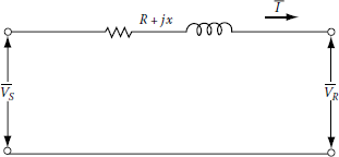
Assume that the circuit shown in Figure 7.5 represents a single-phase circuit if dimensional variables are used; it represents a balanced three-phase circuit if per unit variables are used. R + jX represents the total impedance of lines and/or transformers. The power factor of the load is cosθ = cos(θVR – θT). Find the load power factor for which the voltage drop is maximum.

Solution

The line voltage drop is

$\text{VD}=I\left(R\cos \theta +X\sin \theta \right)$

By taking its partial derivative with respect to the θ angle and equating the result to zero,

$\frac{\partial (\text{VD})}{\partial \theta }=I\left(R\cos \theta +X\sin \theta \right)=0$

or

$\frac{X}{R}=\frac{\sin \theta }{\cos \theta }=\tan \theta$

therefore

${\theta }_{\max }={\tan }^{-1}\frac{X}{R}$

and from the impedance triangle shown in Figure 7.6, the load power factor for which the voltage drop is maximum is

$\begin{array}{cc}\text{PF}=\text{cos}{\theta }_{\text{max}}=\frac{R}{{\left(R^2+X^2\right)}^{1/2}}\hfill & (7.51)\hfill \end{array}$

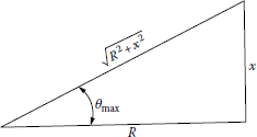
also

$\begin{array}{cc}\cos {\theta }_{\max }=\cos \left({\tan }^{-1}\frac{X}{R}\right)\hfill & (7.52)\hfill \end{array}$

Example 7.5

Consider the three-phase four-wire 416-V secondary system with balanced per-phase loads at A, B, and C as shown in Figure 7.7. Determine the following:

1. Calculate the total voltage drop, or as it is sometimes called, voltage regulation, in one phase of the lateral by using the approximate method.
2. Calculate the real power per phase for each load.
3. Calculate the reactive power per phase for each load.
4. Calculate the total (three-phase) kilovoltampere output and load power factor of the distribution transformer.

Solution

1. Using the approximate voltage-drop equation, that is,

   $\text{VD}=I\left(R\cos \theta +X\sin \theta \right)$

   the voltage drop for each load can be calculated as

   $\begin{array}{ccc}{\text{VD}}_A\hfill & =\hfill & 30\left(0.05\times 1.0+0.01\times 0\right)=1.5\text{V}\hfill \\ {\text{VD}}_{\text{B}}\hfill & =\hfill & 20\left(0.15\times 0.5+0.03\times 0.866\right)=2.02\text{V}\hfill \\ {\text{VD}}_{\text{C}}\hfill & =\hfill & 50\left(0.20\times 0.9+0.08\times 0.436\right)=10.744\text{V}\hfill \end{array}$

   Therefore, the total voltage drop is

   $\begin{array}{lll}{\displaystyle \sum \text{VD}}\hfill & =\hfill & {\text{VD}}_A+{\text{VD}}_{\text{B}}+{\text{VD}}_{\text{C}}\hfill \\ \hfill & =\hfill & 1.5+2.02+10.744\hfill \\ \hfill & =\hfill & 14.264\text{V}\hfill \end{array}$

   or

   $\frac{14.264\text{V}}{240\text{V}}=0.0594\text{pu}\text{V}$

2. The per-phase real power for each load can be calculated from

   $P=VI\cos \theta$

   or

   $\begin{array}{lllll}{P}_A\hfill & =\hfill & 240\times 30\times 1.0\hfill & =\hfill & 7.2\text{kW}\hfill \\ P_B\hfill & =\hfill & 240\times 20\times 0.5\hfill & =\hfill & 2.4\text{kW}\hfill \\ P_C\hfill & =\hfill & 240\times 50\times 0.9\hfill & =\hfill & 10.8\text{kW}\hfill \end{array}$

   Therefore, the total per-phase real power is

   $\begin{array}{lll}{\displaystyle \sum P}\hfill & =\hfill & P_A+P_B+P_C\hfill \\ \hfill & =\hfill & 7.2+2.4+10.8\hfill \\ \hfill & =\hfill & 20.4\text{kW}\hfill \end{array}$

3. The reactive power per phase for each load can be calculated from

   $Q=VI\sin \theta$

   or

   $\begin{array}{lll}{Q}_A\hfill & =\hfill & 240\times 30\times 0=0\text{kvar}\hfill \\ Q_B\hfill & =\hfill & 240\times 20\times 0.866=4.156\text{kvar}\hfill \\ Q_C\hfill & =\hfill & 240\times 50\times 0.436=5.232\text{kvar}\hfill \end{array}$

   Therefore, the total per-phase reactive power is

   $\begin{array}{lll}{\displaystyle \sum Q}\hfill & =\hfill & Q_A+Q_B+Q_C\hfill \\ \hfill & =\hfill & 0+4.156+5.232\hfill \\ \hfill & =\hfill & 9.389\text{kvar}\hfill \end{array}$

4. Therefore, the per-phase kilovoltampere output of the distribution transformer is

   $\begin{array}{lll}S\hfill & =\hfill & {\left(P^2+Q^2\right)}^{1/2}\hfill \\ \hfill & =\hfill & {\left({20.4}^2+{9.389}^2\right)}^{1/2}\hfill \\ \hfill & \cong \hfill & 22.457\text{kVA/phase}\hfill \end{array}$

   Thus the total (or three-phase) kilovoltampere output of the distribution transformer is

   $3\times 22.457=67.37\text{kVA}$

   Hence, the load power factor of the distribution transformer is

   $\begin{array}{lll}\cos \theta \hfill & =\hfill & \frac{{\displaystyle \sum P}}{S}\hfill \\ \hfill & =\hfill & \frac{20.4\text{kW}}{22.457\text{kVA}}\hfill \\ \hfill & =\hfill & 0.908\text{lagging}\hfill \end{array}$

Example 7.6

This example is a continuation of Example 6.1. It deals with voltage drops in the secondary distribution system. In this and the following examples, a single-phase three-wire 120/240 V directly buried underground residential distribution (URD) secondary system will be analyzed, and calculations will be made for motor-starting voltage dip (VDIP) and for steady-state voltage drops at the time of annual peak load. Assume that the cable impedances given in Table 7.2 are correct for a typical URD secondary cable.

Transformer data. The data given in Table 7.1 are for modern single-phase 65°C OISC distribution transformers of the 7200-120/240 V class. The data were taken from a recent catalog of a manufacturer. All given per unit values are based on the transformer-rated kilovoltamperes and voltages.

The 2400 V-class transformers of the sizes being considered have about 15% less R and about 7% less X than the 7200 V transformers. Ignore the small variation of impedance with rated voltage and assume that voltage drop calculated with the given data will suffice for whichever primary voltage is used.

URD secondary cable data. Cable insulations and manufacture are constantly being improved, especially for high-voltage cables. Therefore, any cable data soon become obsolete. The following information and data have been abstracted from recent cable catalogs.

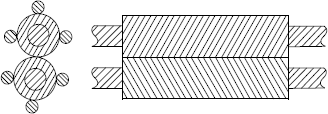
Much of the 600 V-class cables now commonly used for secondary lines (SLs) and services have Al conductor and cross-linked PE insulation, which can stand 90°C conductor temperature. The triplexed cable assembly shown in Figure 7.8 (quadruplexed for three-phase four-wire service) has three or four insulated conductors when aluminum is used. When copper is used, the one grounded neutral conductor is bare. The neutral conductor typically is two AWG sizes smaller than the phase conductors.

The twin concentric cable assembly shown in Figure 7.9 has two insulated copper or aluminum phase conductors plus several spirally served small bare copper binding conductors that act as the current-carrying grounded neutral. The number and size of the spiral neutral wires vary so that the ampacity of the neutral circuit is equivalent to two AWG wire sizes smaller than the phase conductors. Table 7.2 gives data for twin concentric aluminum/copper XLPE 600 V-class cable.

The triplex and twin concentric assemblies obviously have the same resistance for a given size of phase conductors. The triplex assembly has very slightly higher reactance than the concentric assembly. The difference in reactances is too small to be noted unless precise computations are undertaken for some special purpose. The reactances of those cables should be increased by about 25% if they are installed in iron conduit. The reactances given in the following text are valid only for balanced loading (where the neutral current is zero).

The triplex assembly has about 15% smaller ampacity than the concentric assembly, but the exact amount of reduction varies with wire size. The ampacities given are for 90°C conductor temperature, 20°C ambient earth temperature, direct burial in earth, and 10% daily load factor. When installed in buried duct, the ampacities are about 70% of those listed later. For load factors less than 100%, consult current literature or cable standards. The increased ampacities are significantly large.

Arbitrary criteria

1. Use the approximate voltage-drop equation, that is,

   $\text{VD}=I\left(R\cos \theta +X\sin \theta \right)$

   and adapt it to per unit data when computing transformer voltage drops and adapt it to ampere and ohm data when computing SD and SL voltage drops. Obtain all voltage-drop answers in per unit based on 240 V.

2. Maximum allowable motor-starting VDIP = 3% = 0.03 pu = 3.6 V based on 120 V. This figure is arbitrary; utility practices vary.
3. Maximum allowable steady-state voltage drop in the secondary system (transformer + SL + SD) = 3.50% = 0.035 pu = 4.2 V based on 120 V. This figure also is quite arbitrary; regulatory commission rules and utility practices vary. More information about favorable and tolerable amounts of voltage drop will be discussed in connection with subsequent examples, which will involve voltage drops in the primary lines.
4. The loading data for the computation of steady-state voltage drop is given in Table 7.3.
5. As loading data for transient motor-starting VDIP, assume an air-conditioning compressor motor located most unfavorably. It has a 3 hp single-phase 240 V 80 A locked rotor current, with a 50% PF locked rotor.

Assumptions

1. Assume perfectly balanced loading in all three-wire single-phase circuits.
2. Assume nominal operating voltage of 240 V when computing currents from kilovoltampere loads.
3. Assume 90% lagging power factor for all loads.

Using the given data and assumptions, calculate the $\tilde{K}$ constant for any one of the secondary cable sizes, hoping to verify one of the given values in Table 7.2.

Solution

Let the secondary cable size be #2 AWG, arbitrarily. Also let the I current be 100 A and the length of the SL be 100 ft. Using the values from Table 7.2, the resistance and reactance values for 100 ft of cable can be found as

$\begin{array}{lll}R\hfill & =\hfill & 0.334\Omega /1000\text{ft}\times \frac{100\text{ft}}{1000\text{ft}}\hfill \\ \hfill & =\hfill & 0.0334\Omega \hfill \end{array}$

and

$\begin{array}{lll}X\hfill & =\hfill & 0.0299\Omega /1000\text{ft}\times \frac{100\text{ft}}{1000\text{ft}}\hfill \\ \hfill & =\hfill & 0.00299\Omega \hfill \end{array}$

Therefore, using the approximate voltage-drop equation,

$\begin{array}{lll}\text{VD}\hfill & =\hfill & I\left(R\cos \theta +X\sin \theta \right)\hfill \\ \hfill & =\hfill & 100\left(0.0334\times 0.9+0.00299\times 0.435\right)\hfill \\ \hfill & =\hfill & 3.136\text{V}\hfill \end{array}$

or, in per unit volts,

$\frac{3.136\text{V}}{120\text{V}}=0.0261\text{pu}\text{V}$

which is very close to the value given in Table 7.2 for the $\tilde{K}$ constant, that is, 0.02613 pu V/(104A · ft) of cable.

Example 7.7

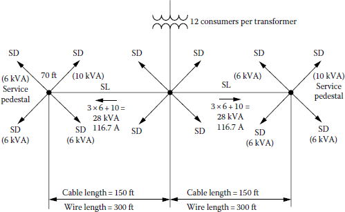
Use the information and data given in Examples 6.1 and 7.3. Assume a URD system. Therefore, the SLs shown in Figure 6.12 are made of UG secondary cables. Assume 12 services per distribution transformer and two transformers per block that are at the locations of poles 2 and 5, as shown in Figure 6.12. Service pedestals are at the locations of poles 1, 3, 4, and 6. Assume that the selected equipment sizes (for ST, ASL, ASD) are of the nearest standard size that are larger than the theoretically most economical sizes and determine the following:

1. Find the steady-state voltage drop in per units at the most remote consumer’s meter for the annual maximum system loads given in Table 7.3.
2. Find the VDIP in per units for motor starting at the most unfavorable location.
3. If the voltage-drop and/or VDIP criteria are not met, select larger equipment and find a design that will meet these arbitrary criteria. Do not, however, immediately select the largest sizes of ST, ASL, and ASD equipment and call that a worthwhile design. In addition, contemplate the data and results and attempt to be wise in selecting ASL or ASD (or both) for enlarging to meet the voltage criteria.

Solution

1. Due to the diversity factors involved, the load values given in Table 7.3 are different for SDs, SLs, and transformers. For example, the load on the transformer is selected as

   $\begin{array}{lll}\text{Transformer}\text{load}\hfill & =\hfill & 10+11\times 4.4\hfill \\ \hfill & =\hfill & 58.4\text{kVA}\hfill \end{array}$

   Therefore, selecting a 50 kVA transformer,

   $\begin{array}{lll}I\hfill & =\hfill & \frac{58.4\text{kVA/240}\text{V}}{S_r/240\text{V}}\hfill \\ \hfill & =\hfill & \frac{58.4\text{kVA}}{50\text{kVA}}\hfill \\ \hfill & =\hfill & 1.168\text{pu}\text{A}\hfill \end{array}$

   Thus, the per unit voltage drop in the transformer is

   $\begin{array}{lll}{\text{VD}}_T\hfill & =\hfill & I\left(R\cos \theta +X\sin \theta \right)\hfill \\ \hfill & =\hfill & \left(1.168\text{pu}\text{A}\right)\left(0.0107\times 0.9+0.0139\times 0.435\right)\hfill \\ \hfill & =\hfill & 0.0183\text{pu}\text{V}\hfill \end{array}$

   As shown in Figure 7.10, the load on each SL (that portion of the wiring between the transformer and the service pedestal) is similarly calculated as

   $\begin{array}{lll}\text{SL}\text{load}\hfill & =\hfill & 10+3\times 6\hfill \\ \hfill & =\hfill & 28\text{kVA}\hfill \end{array}$

   Figure 7.10

   

   Circulation of the secondary-line currents.

   or 116.7 A. If the SL is selected to be #4/0 AWG with the $\tilde{K}$ constant of 0.0088 from Table 7.2, the per unit voltage drop in each SL is

   $\begin{array}{lll}{\text{VD}}_{\text{SL}}\hfill & =\hfill & \tilde{K}\left(\frac{I\times l}{{10}^4}\right)\hfill \\ \hfill & =\hfill & 0.0088\left(\frac{116.7\times 150\text{ft}}{{10}^4}\right)\hfill \\ \hfill & =\hfill & 0.01554\text{pu}\text{V}\hfill \end{array}$

   The load on each SD is given to be 10 kVA or 41.6 A from Table 7.3. If each SD of 70 ft length is selected to be #1/0 AWG with the $\tilde{K}$ constant of 0.01683 from Table 7.2, the per unit voltage drop in each SD is

   $\begin{array}{lll}{\text{VD}}_{\text{SD}}\hfill & =\hfill & \tilde{K}\left(\frac{I\times l}{{10}^4}\right)\hfill \\ \hfill & =\hfill & 0.01683\left(\frac{41.6\text{A}\times 70\text{ft}}{{10}^4}\right)\hfill \\ \hfill & =\hfill & 0.0049\text{puV}\hfill \end{array}$

   Therefore, the total steady-state voltage drop in per units at the most remote consumer’s meter is

   $\begin{array}{lll}{\displaystyle \sum \text{VD}}\hfill & =\hfill & {\text{VD}}_T+{\text{VD}}_{\text{SL}}+{\text{VD}}_{\text{SD}}\hfill \\ \hfill & =\hfill & 0.0183+0.01554+0.0049\hfill \\ \hfill & =\hfill & 0.0388\text{pu}\text{V}\hfill \end{array}$

   which exceeds the given criterion of 0.035 pu V.

2. To find the VDIP in per units for motor starting at the most unfavorable location, the given starting current of 80 A can be converted to a kilovoltampere load of 19.2 kVA (80 A × 240 V). Therefore, the per unit VDIP in the 50 kVA transformer is

   $\begin{array}{lll}{\text{VDIP}}_T\hfill & =\hfill & \left(R\cos \theta +X\sin \theta \right)\left(\frac{19.2\text{kVA}}{50\text{kVA}}\right)\hfill \\ \hfill & =\hfill & \left(0.0107\times 0.5+0.0139\times 0.866\right)\left(\frac{19.2\text{kVA}}{50\text{kVA}}\right)\hfill \\ \hfill & =\hfill & 0.00668\text{pu}\text{V}\hfill \end{array}$

   The per unit VDIP in the SL of #4/0 AWG cable is

   $\begin{array}{lll}{\text{VDIP}}_{\text{SL}}\hfill & =\hfill & \tilde{K}\left(\frac{80\text{A}\times 150\text{ft}}{{10}^4}\right)\hfill \\ \hfill & =\hfill & 0.00636\left(\frac{80\times 150}{{10}^4}\right)\hfill \\ \hfill & =\hfill & 0.00763\text{pu}\text{V}\hfill \end{array}$

   The per unit VDIP in the SD of #1/0 AWG cable is

   $\begin{array}{lll}{\text{VDIP}}_{\text{SD}}\hfill & =\hfill & \tilde{K}\left(\frac{80\text{A}\times 70\text{ft}}{{10}^4}\right)\hfill \\ \hfill & =\hfill & 0.01089\left(\frac{80\times 70}{{10}^4}\right)\hfill \\ \hfill & =\hfill & 0.0061\text{pu}\text{V}\hfill \end{array}$

   Therefore, the total VDIP in per units due to motor starting at the most unfavorable location is

   $\begin{array}{lll}{\displaystyle \sum \text{VDIP}}\hfill & =\hfill & {\text{VDIP}}_T+{\text{VDIP}}_{\text{SL}}+{\text{VDIP}}_{\text{SD}}\hfill \\ \hfill & =\hfill & 0.00668+0.00763+0.0061\hfill \\ \hfill & =\hfill & 0.024\text{pu}\text{V}\hfill \end{array}$

   which meets the given criterion of 0.03 pu V.

3. Since in part (a) the voltage-drop criterion has not been met, select the SL cable size to be one size larger than the previous #4/0 AWG size, that is, 250 kcmil, keeping the size of the transformer the same. Therefore, the new per unit voltage drop in the SL becomes

   $\begin{array}{lll}{\text{VD}}_{\text{SL}}\hfill & =\hfill & 0.00769\left(\frac{116.7\text{A}\times 150\text{ft}}{{10}^4}\right)\hfill \\ \hfill & =\hfill & 0.01347\text{pu}\text{V}\hfill \end{array}$

   Also, selecting one-size-larger cable, that is, #2/0 AWG, for the SD, the new per unit voltage drop in the SD becomes

   $\begin{array}{lll}{\text{VD}}_{\text{SD}}\hfill & =\hfill & 0.0136\left(\frac{41.6\text{A}\times 70\text{ft}}{{10}^4}\right)\hfill \\ \hfill & =\hfill & 0.00396\text{pu}\text{V}\hfill \end{array}$

   Therefore, the new total steady-state voltage drop in per units at the most remote consumer’s meter is

   $\begin{array}{lll}\text{VD}\hfill & =\hfill & {\text{VD}}_T+{\text{VD}}_{\text{SL}}+{\text{VD}}_{\text{SD}}\hfill \\ \hfill & =\hfill & 0.0183+0.01347+0.00396\hfill \\ \hfill & =\hfill & 0.03573\text{pu}\text{V}\hfill \end{array}$

   which is still larger than the criterion. Thus, select 350 kcmil cable size for the SLs and #2/0 AWG cable size for the SDs to meet the criteria.

Example 7.8

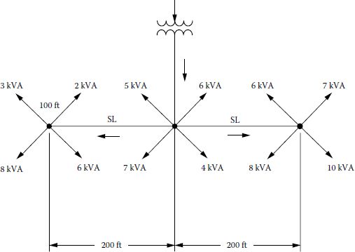
Figure 7.11 shows a residential secondary distribution system. Assume that the distribution transformer capacity is 75 kVA (use Table 7.1), all secondaries and services are single-phase three wire, nominally 120/240 V, and all SLs are of #2/0 A1/Cu XLPE cable, and SDs are of #1/0 Al/Cu XLPE cable (use Table 7.2). All SDs are 100 ft long, and all SLs are 200 ft long. Assume an average lagging-load power factor of 0.9 and 100% load diversity factors and determine the following:

1. Find the total load on the transformer in kilovoltamperes and in per units.
2. Find the total steady-state voltage drop in per units at the most remote and severe customer’s meter for the given annual maximum system loads.

Solution

1. Assuming a diversity factor of 100%, the total load on the transformer is

   $\begin{array}{lll}{S}_T\hfill & =\hfill & \left(3+2+8+6\right)\left(5+6+7+4\right)\left(6+7+8+10\right)\hfill \\ \hfill & =\hfill & 19+22+31\hfill \\ \hfill & =\hfill & 72\text{kVA}\hfill \end{array}$

   or, in per units,

   $\begin{array}{lll}I\hfill & =\hfill & \frac{S_r}{S_B}\hfill \\ \hfill & =\hfill & \frac{72\text{kVA}}{75\text{KVA}}\hfill \\ \hfill & =\hfill & 0.96\text{pu}\text{A}\hfill \end{array}$

2. To find the total voltage drop in per units at the most remote and severe customer’s meter, calculate the per unit voltage drops in the transformer, the service line, and the SD of the most remote and severe customer. Therefore,

   $\begin{array}{lll}{\text{VD}}_{\text{r}}\hfill & =\hfill & I\left(R\cos \theta +X\sin \theta \right)\hfill \\ \hfill & =\hfill & 0.96\left(0.0101\times 0.90+0.0143\times 0.4359\right)\hfill \\ \hfill & =\hfill & 0.0147\text{pu}\text{V}\hfill \end{array}$

   $\begin{array}{lll}{\text{VD}}_{\text{SL}}\hfill & =\hfill & \tilde{K}\left(\frac{I\times I}{{10}^4}\right)\hfill \\ \hfill & =\hfill & 0.0136\left(\frac{129.17\text{A}\times 200\text{ft}}{{10}^4}\right)\hfill \\ \hfill & =\hfill & 0.03513\text{pu}\text{V}\hfill \end{array}$

   $\begin{array}{lll}{\text{VD}}_{\text{SD}}\hfill & =\hfill & \tilde{K}\left(\frac{I\times I}{{10}^4}\right)\hfill \\ \hfill & =\hfill & 0.01683\left(\frac{41.67\text{A}\times 100\text{ft}}{{10}^4}\right)\hfill \\ \hfill & =\hfill & 0.0070\text{pu}\text{V}\hfill \end{array}$

   Therefore, the total voltage drop is

   $\begin{array}{lll}{\displaystyle \sum \text{VD}}\hfill & =\hfill & {\text{VD}}_T+{\text{VD}}_{\text{SL}}+{\text{VD}}_{\text{SD}}\hfill \\ \hfill & =\hfill & 0.0147+0.03513+0.0070\hfill \\ \hfill & =\hfill & 0.0568\text{pu}\text{V}\hfill \end{array}$

Example 7.9

Figure 7.12 shows a three-phase four-wire grounded-wye distribution system with multigrounded neutral, supplied by an express feeder and mains. In the figure, d and s are the width and length of a primary lateral, where s is much larger than d. Main lengths are equal to cb = ce = s/2. The number of the primary laterals can be found as s/d. The square-shaped service area (s2) has a uniformly distributed load density, and all loads are presumed to have the same lagging power factor. Each primary lateral, such as ba, serves an area of length s and width d. Assume that

• D = uniformly distributed load density, kVA/(unit length)2
• VL-L = nominal operating voltage, which is also the base voltage, line-to-line kV
• rm + jxm = impedance of three-phase express and mains, Ω/(phase · unit length)
• rl + jxl = impedance of a three-phase lateral line, Ω/(phase · unit length)

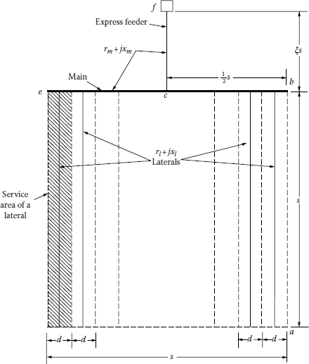
Use the given information and data and determine the following:

1. 1. Assume that the laterals are in three phase and find the per unit voltage-drop expressions for
   1. The express feeder fc, that is, VDpu,fc
   2. The main cb, that is, VDpu,cb

   3. The primary lateral ba, that is, VDpu,ba

      Note that the equations to be developed should contain the constants D, s, d, impedances, θ, load power-factor angle, VL-L, etc., but not current variable I.

2. 2. Change all the laterals from the three-phase four-wire system to an open-wye system so that investment costs will be reduced, but three-phase secondary service can still be rendered where needed. Assume that the phasing connections of the many laterals are well balanced on the mains. Use Morrison’s approximations and modify the equations derived in part (1).

Solution

1. 1.

   $\begin{array}{cc}\text{Total}\text{kVA}\text{load served}=D\times s^2\text{kVA}\hfill & (7.53)\hfill \end{array}$

   $\begin{array}{cc}\text{Current}\text{at}\text{point}f=\frac{D\times s^2}{\sqrt{3}\times V_{L-L}}\hfill & (7.54)\hfill \end{array}$

   $\begin{array}{cc}\text{Voltage}\text{drop}=I\times Z\times I_{eff}\hfill & (7.55)\hfill \end{array}$

   Therefore,

   1. $\begin{array}{llll}{\text{VD}}_{\text{pu,}fc}\hfill & =\hfill & \frac{D\times s^2}{\sqrt{3}\times V_{L-L}}\left(r_m\cos \theta +X_m\sin \theta \right)\frac{\sqrt{3}}{1000\times V_{L-L}}\left(\zeta \times s\right)\hfill & \hfill \\ \hfill & =\hfill & \frac{\zeta \times D\times s^3}{1000\times V^2{}_{L-L}}\left(r_m\cos \theta +X_m\sin \theta \right)\hfill & (7.56)\hfill \end{array}$
   2. $\begin{array}{llll}{\text{VD}}_{\text{pu,}cb}\hfill & =\hfill & \frac{\frac{1}{2}D\times s^2}{\sqrt{3}\times V_{L-L}}\left(r_m\cos \theta +X_m\sin \theta \right)\frac{\sqrt{3}}{1000\times V_{L-L}}\left(\frac{1}{4}\times s\right)\hfill & \hfill \\ \hfill & =\hfill & \frac{D\times s^3}{8000\times V_{L-L}^2}\left(r_m\cos \theta +X_m\sin \theta \right)\hfill & (7.57)\hfill \end{array}$

   3. $\begin{array}{llll}{\text{VD}}_{\text{pu,}ba}\hfill & =\hfill & \frac{D\left(d\times s\right)}{\sqrt{3}\times V_{L-L}}\left(r_1\cos \theta +X_1\sin \theta \right)\frac{\sqrt{3}}{1000\times V_{L-L}}\left(\frac{1}{2}\times s\right)\hfill & \hfill \\ \hfill & =\hfill & \frac{D\times d\times s^2}{2000\times V^2{}_{L-L}}\left(r_1\cos \theta +X_1\sin \theta \right)\hfill & (7.58)\hfill \end{array}$

2. 2. There would not be any change in the equations given in part (1).

Example 7.10

Figure 7.13 shows a square-shaped service area (A = 4 mi2) with a uniformly distributed load density of D kVA/mi2 and 2 mi of #4/0 AWG copper overhead main from a to b. There are many closely spaced primary laterals that are not shown in the square-shaped service area of the figure. In this voltage-drop study, use the precalculated voltage-drop curves of Figure 4.17 when applicable. Use the nominal primary voltage of 7,620/13,200 V for a three-phase four-wire wye-grounded system. Assume that at peak loading, the load density is 1000 kVA/mi2 and the lumped load is 2000 kVA, and that at off-peak loading, the load density is 333 kVA/mi2 and the lumped load is still 2000 kVA. The lumped load is of a small industrial plant working three shifts a day. The substation bus voltages are 1.025 pu V of 7620 base volts at peak load and 1.000 pu V during off-peak load.

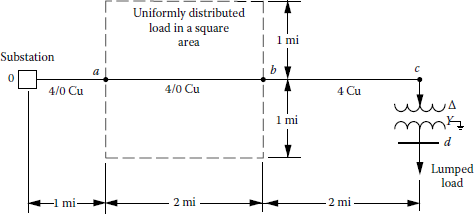
The transformer located between buses c and d has a three-phase rating of 2000 kVA and a delta-rated high voltage of 13,200 V and grounded-wye-rated low voltage of 277/480 V. It has 0 + j0.05 per unit impedance based on the transformer ratings. It is tapped up to raise the low voltage 5.0% relative to the high voltage, that is, the equivalent turns ratio in use is (7620/277) × 0.95. Use the given information and data for peak loading and determine the following:

1. The percent voltage drop from the substation to point a, from a to b, from b to c, and from c to d on the main
2. The per unit voltages at the points a, b, c, and d on the main
3. The line-to-neutral voltages at the points a, b, c, and d

Solution

1. The load connected in the square-shaped service area is

   $\begin{array}{lll}{S}_n\hfill & =\hfill & D\times A_n\hfill \\ \hfill & =\hfill & 1000\times 4\hfill \\ \hfill & =\hfill & 4000\text{kVA}\hfill \end{array}$

   Thus the total kilovoltampere load on the main is

   $\begin{array}{lll}{S}_m\hfill & =\hfill & 4000+2000\hfill \\ \hfill & =\hfill & 6000\text{kVA}\hfill \end{array}$

   From Figure 4.17, for #4/0 copper, the K constant is found to be 0.0003. Therefore, the percent voltage drop from the substation to point a is

   $\begin{array}{lll}\%{\text{VD}}_{\text{0a}}\hfill & =\hfill & K\times S_m\times 1\hfill \\ \hfill & =\hfill & 0.0003\times 6000\times 1\hfill \\ \hfill & =\hfill & 148\%\text{V}\text{or}0.018\text{pu}\text{V}\hfill \end{array}$

   The percent voltage drop from point a to point b is

   $\begin{array}{lll}\%{\text{VD}}_{\text{ab}}\hfill & =\hfill & K\times S_n\times 1+K\times S_{\text{lump}}\times 1\hfill \\ \hfill & =\hfill & 0.0003\times 4000\times 1+0.0003\times 2000\times 2\hfill \\ \hfill & =\hfill & 2.4\%\text{V}\text{or}0.024\text{pu}\text{V}\hfill \end{array}$

   The percent voltage drop from point b to point c is

   $\begin{array}{lll}\%{\text{VD}}_{\text{bc}}\hfill & =\hfill & K\times S_{\text{lump}}\times I\hfill \\ \hfill & =\hfill & 0.0009\times 2000\times 2\hfill \\ \hfill & =\hfill & 3.6\%\text{V}\text{or}0.036\text{pu}\text{V}\hfill \end{array}$

   To find the percent voltage drop from point c to bus d,

   $\begin{array}{lll}I\hfill & =\hfill & \frac{2000\text{kVA}}{\sqrt{3}\times V_{L-L}\text{at}\text{point}c}\hfill \\ \hfill & =\hfill & \frac{2000\text{kVA}}{\sqrt{3}\times \left(0.947\times 13.2\text{V}\right)}\hfill \\ \hfill & =\hfill & 92.373\text{A}\hfill \end{array}$

   $\begin{array}{lll}{I}_B\hfill & =\hfill & \frac{2000\text{kVA}}{\sqrt{3}\times 13.2\text{kV}}\hfill \\ \hfill & =\hfill & 87.477\text{A}\hfill \end{array}$

   $\begin{array}{lll}{I}_{\text{pu}}\hfill & =\hfill & \frac{I}{I_B}\hfill \\ \hfill & =\hfill & 1.056\text{pu}\text{A}\hfill \end{array}$

   Note that usually in a simple problem like this, the reduced voltage at point c is ignored. In that case, for example, the per unit current would be 1.0 pu A rather than 1.056 pu A. Since

   $Z_{T,\text{pu}}=0+j0.05\text{pu}\Omega$

   and

   $\cos \theta =0.9or\theta ={25.84}^{\circ }\text{lagging}$

   therefore

   $I_{p\text{u}}=1.056\angle {25.84}^{\circ }\text{pu}\text{A}$

   Thus, to find the percent voltage drop at bus d, first it can be found in per unit as

   ${\text{VD}}_{\text{cd}}=\frac{I\left(R\cos \theta +X\sin \theta \right)}{V_B}\text{pu}\text{V}$

   but since the low voltage has been tapped up 5%,

   ${\text{VD}}_{\text{cd}}=\frac{I\left(R\cos \theta +X\sin \theta \right)}{V_B}-0.05\text{pu}\text{V}$

   Therefore,

   $\begin{array}{lll}{\text{VC}}_{cd}\hfill & =\hfill & \frac{1.056\left(0\times 0.9+0.05\times 0.4359\right)}{1.0}-0.05\hfill \\ \hfill & =\hfill & -0.0267\text{pu}\text{V}\hfill \end{array}$

   or

   $\%{\text{VD}}_{cd}=-2.67\%\text{V}$

   Here, the negative sign of the voltage drop indicates that it is in fact a voltage rise rather than a voltage drop.

2. The per unit voltages at the points a, b, c, and d on the main are

   $\begin{array}{lll}{V}_a\hfill & =\hfill & V_0-V_{0a}\hfill \\ \hfill & =\hfill & 1.025-0.018\hfill \\ \hfill & =\hfill & 1.007\text{pu}\text{V}\text{or}100\text{.7\%}\text{V}\hfill \end{array}$

   $\begin{array}{lll}{V}_b\hfill & =\hfill & V_a-V_{ab}\hfill \\ \hfill & =\hfill & 1.007-0.024\hfill \\ \hfill & =\hfill & 0.983\text{pu}\text{V}\text{or}98\text{.3\%}\text{V}\hfill \end{array}$

   $\begin{array}{lll}{V}_c\hfill & =\hfill & V_b-V_{bc}\hfill \\ \hfill & =\hfill & 0.983-0.036\hfill \\ \hfill & =\hfill & 0.947\text{pu}\text{V}\text{or}94\text{.7\%}\text{V}\hfill \end{array}$

   $\begin{array}{lll}{V}_d\hfill & =\hfill & V_c-V_{cd}\hfill \\ \hfill & =\hfill & 0.947-\left(-0.0267\right)\hfill \\ \hfill & =\hfill & 0.9737\text{pu}\text{V}\text{or}97\text{.37\%}\text{V}\hfill \end{array}$

3. The line-to-neutral voltages are

   $\begin{array}{lll}{V}_a\hfill & =\hfill & 7620\times 1.007\hfill \\ \hfill & =\hfill & 7673.3\text{V}\hfill \end{array}$

   $\begin{array}{lll}{V}_b\hfill & =\hfill & 7620\times 0.983\hfill \\ \hfill & =\hfill & 7490.5\text{V}\hfill \end{array}$

   $\begin{array}{lll}{V}_c\hfill & =\hfill & 7620\times 0.947\hfill \\ \hfill & =\hfill & 7216.1\text{V}\hfill \end{array}$

   $\begin{array}{lll}{V}_d\hfill & =\hfill & 277\times 0.9737\hfill \\ \hfill & =\hfill & 269.7\text{V}\hfill \end{array}$

Example 7.11

Use the relevant information and data given in Example 7.10 for off-peak loading and repeat Example 7.10, and find the Vd voltage at bus d in line-to-neutral volts. Also write the necessary codes to solve the problem in MATLAB.

Solution

1. At off-peak loading, the load connected in the square-shaped service area is

   $\begin{array}{lll}{S}_n\hfill & =\hfill & D\times A_n\hfill \\ \hfill & =\hfill & 333\times 4\hfill \\ \hfill & =\hfill & 1332\text{kVA}\hfill \end{array}$

   Thus the total kilovoltampere load on the main is

   $\begin{array}{lll}{S}_m\hfill & =\hfill & 1332+2000\hfill \\ \hfill & =\hfill & 3332\text{kVA}\hfill \end{array}$

   Therefore, the percent voltage drop from the substation to point a is

   $\begin{array}{lll}\%{\text{VD}}_{0a}\hfill & =\hfill & K\times S_m\times 1\hfill \\ \hfill & =\hfill & 0.0003\times 3332\times 1\hfill \\ \hfill & =\hfill & 10\%\text{V}\text{or}0.01\text{pu}\text{V}\hfill \end{array}$

   The percent voltage drop from point a to point b is

   $\begin{array}{lll}\%{\text{VD}}_{ab}\hfill & =\hfill & K\times S_n\times 1/2+K\times S_{\text{lump}}\times 1\hfill \\ \hfill & =\hfill & 0.003\times 1332\times 1+0.0003\times 2000\times 2\hfill \\ \hfill & =\hfill & 1.6\%\text{V}\text{or}0.016\text{pu}\text{V}\hfill \end{array}$

   The percent voltage drop from point b to point c is

   $\begin{array}{lll}{\text{VD}}_{bc}\hfill & =\hfill & K\times S_{\text{lump}}\times I\hfill \\ \hfill & =\hfill & 0.0009\times 2000\times 2\hfill \\ \hfill & =\hfill & 3.6\%\text{V}\text{or}0.036\text{pu}\text{V}\hfill \end{array}$

   To find the percent voltage drop from point c to bus d, the percent voltage drop at bus d can be found as before

   $\%{\text{VD}}_{cd}=0.0267\text{pu}\text{V}\text{or}\text{-2}\text{.67\%}\text{V}$

2. The per unit voltages at points a, b, c, and d on the main are

   $\begin{array}{lll}{V}_a\hfill & =\hfill & V_0-V_{0a}\hfill \\ \hfill & =\hfill & 1.0-0.01\hfill \\ \hfill & =\hfill & 0.99\text{pu}\text{V}\text{or}\text{99\%}\text{V}\hfill \end{array}$

   $\begin{array}{lll}{V}_b\hfill & =\hfill & V_a-V_{ab}\hfill \\ \hfill & =\hfill & 0.99-0.016\hfill \\ \hfill & =\hfill & 0.974\text{pu}\text{V}\text{or}97\text{.4\%}\text{V}\hfill \end{array}$

   $\begin{array}{lll}{V}_c\hfill & =\hfill & V_b-V_{bc}\hfill \\ \hfill & =\hfill & 0.974-0.036\hfill \\ \hfill & =\hfill & 0.938\text{pu}\text{V}\text{or}93.8\text{\%V}\hfill \end{array}$

   $\begin{array}{lll}{V}_d\hfill & =\hfill & V_c-V_{cd}\hfill \\ \hfill & =\hfill & 0.938-\left(-0.0267\right)\hfill \\ \hfill & =\hfill & 0.9647\text{pu}\text{V}\text{or}96\text{.47\%}\text{V}\hfill \end{array}$

3. The line-to-neutral voltages are

   $\begin{array}{lll}{V}_a\hfill & =\hfill & 7620\times 0.99\hfill \\ \hfill & =\hfill & 7543.8\text{V}\hfill \end{array}$

   $\begin{array}{lll}{V}_b\hfill & =\hfill & 7620\times 0.974\hfill \\ \hfill & =\hfill & 7421.9\text{V}\hfill \end{array}$

   $\begin{array}{lll}{V}_c\hfill & =\hfill & 7620\times 0.938\hfill \\ \hfill & =\hfill & 7147.6\text{V}\hfill \end{array}$

   $\begin{array}{lll}{V}_d\hfill & =\hfill & 277\times 0.9647\hfill \\ \hfill & =\hfill & 267.2\text{V}\hfill \end{array}$

Note that the voltages at bus d during peak and off-peak loading are nearly the same.

Here is the MATLAB script:

clc

clear

% System parameters

St = 2000;% in kVA

D = 1000;% in kVA/mi^2

An = 4;% in mi^2

K40 = 0.0003;% from Figure 4.17 for 4/0 AWG

K4 = 0.0009;% from Figure 4.17 for 4 AWG

L1 = 1;% distanced from substation to point a in miles

L2 = 2;% distanced from point a to b in miles

kV = 13.2;

Xt = 0.05;

PF = 0.9;

Vopu = 1.025;

VBp = 7620;% Voltage base primary

VBs = 277;% Voltage base secondary

% Solution for part a

Sn = D*An

% Total kVA on main

Sm = Sn + St

% Per unit voltage drop from substation to point a

VDoapu = (K40*Sm*L1)/100

% Per unit voltage drop from point a to point b

VDabpu = (K40*Sn*(L2/2)+K40*St*L2)/100

% Per unit voltage drop from point b to point c

VDbcpu = (K4*St*L2)/100

I = St/(sqrt(3)*0.947*kV);

IB = St/(sqrt(3)*kV);

Ipu = I/IB

% Per unit voltage drop from point c to point d

VDcdpu = Ipu*(Xt*sin(acos(PF)))-0.05

% Solution for part b in per units

Vapu = Vopu-VDoapu

Vbpu = Vapu-VDabpu

Vcpu = Vbpu-VDbcpu

Vdpu = Vcpu-VDcdpu

% Solution for part c in per units

Va = Vapu*VBp

Vb = Vbpu*VBp

Vc = Vcpu*VBp

Vd = Vdpu*VBs

Example 7.12

Figure 7.14 shows that a large number of small loads are closely spaced along the length l. If the loads are single phase, they are assumed to be well balanced among the three phases.

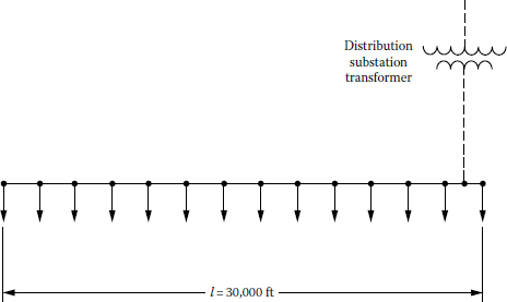
A three-phase four-wire wye-grounded 7.62/13.2 kV primary line is to be built along the length l and fed through a distribution substation transformer from a high-voltage transmission line. Assume that the uniform (or linear) distribution of the connected load along the length l is

$\frac{S_{\text{connected}\text{load}}}{I}=0.45\text{kVA/ft}$

The 30-min annual demand factor of all loads is 0.60, the diversity factor (FD) among all loads is 1.08, and the annual loss factor (FLS) is 0.20. Assuming a lagging power factor of 0.9 for all loads and a 37 in. geometric mean spacing of phase conductors, use Figure 4.17 for voltage-drop calculations for copper conductors. Use the relevant tables in Appendix A for additional data about copper and ACSR conductors and determine the following:

Locate the distribution substation where you think it would be the most economical, considering only the 13.2 kV system, and then find

1. The minimum ampacity-sized copper and ACSR phase conductors
2. The percent voltage drop at the location having the lowest voltage at the time of the annual peak load, using the ampacity-sized copper conductor found in part (a)
3. Also write the necessary codes to solve the problem in MATLAB

Solution

To achieve the minimum voltage drop, the substation should be located at the middle of the line 1, and therefore

1. From Equation 2.13, the diversified maximum demand of the group of the load is

   $\begin{array}{lll}{D}_g\hfill & =\hfill & \frac{{\displaystyle \sum {}_{i-1}^n{\text{TCD}}_{\text{i}}\times {\text{DF}}_{\text{i}}}}{F_D}\hfill \\ \hfill & =\hfill & \frac{0.45\text{kVA/ft}\times 0.60}{1.08}\hfill \\ \hfill & =\hfill & 0.250\text{kVA/ft}\hfill \end{array}$

   Thus the peak load of each main on the substation transformer is

   $\begin{array}{lll}{S}_{PK}\hfill & =\hfill & 0.250\text{kVA/ft}\times \text{15,000}\text{ft}\hfill \\ \hfill & =\hfill & 3750\text{kVA}\hfill \end{array}$

   or

   $3750\text{kVA=}\sqrt{3}\times 13.2\text{kV}\times I$

   hence

   $\begin{array}{lll}I\hfill & =\hfill & \frac{3750\text{kVA}}{\sqrt{3}\times 13.2\text{kV}}\hfill \\ \hfill & =\hfill & 164.2\text{A}\hfill \end{array}$

   in each main out of the substation. Therefore, from the tables of Appendix A, it can be recommended that either #4 AWG copper conductor or #2 AWG ACSR conductor be used.

2. Assuming that #4 AWG copper conductor is used, the percent voltage drop at the time of the annual peak load is

   $\begin{array}{lll}\%\text{VD}\hfill & =\hfill & \left[K\%\text{VD/}\left(\text{kVA}\cdot \text{mi}\right)\right]\times \left[S_{\text{PK}}\text{kVA}\right]\times \frac{I\text{ft}}{2}\frac{1}{5280\text{ft/mi}}\hfill \\ \hfill & =\hfill & 0.0009\times 3750\times \frac{15,000}{2\times 5280}\hfill \\ \hfill & =\hfill & 5.3\%\text{V}\hfill \end{array}$

3. Here is the MATLAB script:

   clc

   clear

   % System parameters

   D = 333;% off-peak load density in kVA/mi^2

   An = 4;% in mi^2

   K40 = 0.0003;% from Figure 4.17 for 4/0 AWG

   K4 = 0.0009;% from Figure 4.17 for 4 AWG

   L1 = 1;% distanced from substation to point a in miles

   L2 = 2;% distanced from point a to b in miles

   St = 2000;% in kVA Vopu = 1.0;

   VBp = 7620;

   VBs = 277;

   % Solution for part a

   Sn = D*An

   % Total kVA on main

   Sm = Sn + St

   % Per unit voltage drop from substation to point a

   VDoapu = (K40*Sm*L1)/100

   % Per unit voltage drop from point a to point b

   VDabpu = (K40*Sn*(L2/2)+K40*St*L2)/100

   % Per unit voltage drop from point b to point c

   VDbcpu = (K4*St*L2)/100

   VDcdpu = -0.027% as before

   % Solution for part b in per units

   Vapu = Vopu-VDoapu

   Vbpu = Vapu-VDabpu

   Vcpu = Vbpu-VDbcpu

   Vdpu = Vcpu-VDcdpu

   % Solution for part c in per units

   Va = Vapu*VBp

   Vb = Vbpu*VBp

   Vc = Vcpu*VBp

   Vd = Vdpu*VBs

Example 7.13

Now suppose that the line in Example 7.12 is arbitrarily constructed with #4/0 AWG ACSR phase conductor and that the substation remains where you put it in part (a). Assume 50°C conductor temperature and find the total annual I2R energy loss (TAELCu), in kilowatthours, in the entire line length.

Solution

The total I2R loss in the entire line length is Therefore,

$\begin{array}{lll}{\displaystyle \sum I^{2}R}\hfill & =\hfill & 3I^2\left(r\times \frac{1}{2}\right)\hfill \\ \hfill & =\hfill & 3{\left(164.2\right)}^2\left(0.592\Omega /\text{mi}\right)\frac{30,000\text{ft}}{2\times 5280\text{ft/mi}}\hfill \\ \hfill & =\hfill & 136,033.729\text{W}\hfill \end{array}$

Therefore, the total I2R energy loss is

$\begin{array}{lll}{\text{TAEL}}_{\text{cu}}\hfill & =\hfill & \left[\left({\displaystyle \sum I^{2}R}\right)F_{\text{LS}}\right]\left(8760\text{h/year}\right)\hfill \\ \hfill & =\hfill & \frac{136,033.729}{{10}^3}\times 0.20\times 8760\hfill \\ \hfill & =\hfill & 238,331.09\text{kWh}\hfill \end{array}$

Example 7.14

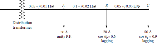
Figure 7.15 shows a single-line diagram of a simple three-phase four-wire wye-grounded primary feeder. The nominal operating voltage and the base voltage are given as 7,200/12,470 V. Assume that all loads are balanced three phase and all have 90% power factor, lagging. The given values of the constant K in Table 7.4 are based on 7,200/12,470 V. There is a total of a 3000 kVA uniformly distributed load over a 4 mi line between b and c. Use the given data and determine the following:

1. Find the total percent voltage drop at points a, b, c, and d.
2. If the substation bus voltages are regulated to 7,300/12,650 V, what are the line-to-neutral and line-to-line voltages at point a?

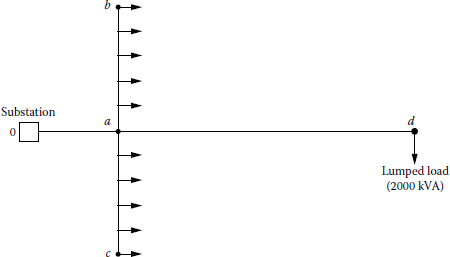
Solution

1. The total load flowing through the line between points 0 and a is

   ${\displaystyle \sum S=2000\text{kVA+3000}\text{kVA}}=5000\text{kVA}$

   therefore the percent voltage drop at point a is

   $\begin{array}{lll}\%{\text{VD}}_{\text{a}}\hfill & =\hfill & K\left({\displaystyle \sum S}\right)I\hfill \\ \hfill & =\hfill & 0.0005\times 5000\times 1.0\hfill \\ \hfill & =\hfill & 2.5\%\text{V}\hfill \end{array}$

   Similarly, the load flowing through the line between points a and b is

   $S=1500\text{kVA}$

   Therefore,

   $\begin{array}{lll}\%{\text{VD}}_b\hfill & =\hfill & K\times S\times I/2+\%{\text{VD}}_a\hfill \\ \hfill & =\hfill & 0.0010\times 1500\times 1+2.5\%\hfill \\ \hfill & =\hfill & 4\%\text{V}\hfill \end{array}$

   $\%{\text{VD}}_c=\%{\text{VD}}_b=4\%\text{V}$

   $\begin{array}{lll}\%{\text{VD}}_d\hfill & =\hfill & K\times S_{\text{lump}}\times I+\%{\text{VD}}_a\hfill \\ \hfill & =\hfill & 0.0010\times 2000\times 2+2.5\%\hfill \\ \hfill & =\hfill & 6.5\%\text{V}\hfill \end{array}$

2. If the substation bus voltages are regulated to 7,300/12,650 V at point a, the line-to-neutral voltage is

   $\begin{array}{lll}{V}_{a,L-N}\hfill & =\hfill & 7300-{\text{VD}}_{a,L-N}\hfill \\ \hfill & =\hfill & 7300-7300\times 0.025\hfill \\ \hfill & =\hfill & 7117.5\text{V}\hfill \end{array}$

   and the line-to-line voltage is

   $\begin{array}{lll}{V}_{a,L-L}\hfill & =\hfill & 12,650-{\text{VD}}_{a,L-L}\hfill \\ \hfill & =\hfill & 12,650-12,650\times 0.025\hfill \\ \hfill & =\hfill & 12,333.8\text{V}\hfill \end{array}$