
You access Google Spreadsheets from the Google Docs home page (docs.google.com). All your existing spreadsheet files are listed there, along with your word processing documents and presentations.
To create a new spreadsheet, all you have to do is click the New button and select Spreadsheet. The new spreadsheet opens in its own window on your desktop. Alternatively, you can select New, From Template to create a new spreadsheet based on a predesigned template; this opens Google’s Template Gallery, from which you can make your choice.
Opening an existing spreadsheet file is equally easy. Just click the file’s name on the Google Docs home page, and the spreadsheet window opens.
When you are finished with a spreadsheet, you need to save the file. When you first save a file, you must do so manually—and give the file a name. After this first save, Google automatically resaves the file every time you make a change to the spreadsheet. In essence, this means that you have to save the spreadsheet only once; Google saves all further changes automatically.
To save a new spreadsheet, click the Save button. When the Save Spreadsheet dialog box appears, enter a name for the spreadsheet, and then click the OK button. That’s all there is to it. The spreadsheet is now saved on Google’s servers, and you don’t have to bother resaving it at any future point.
By default, all the spreadsheets you work with in Google Spreadsheets are stored on Google’s servers. You can, however, download files from Google to your computer’s hard drive to work with in Excel. In essence, you’re exporting your Google spreadsheet to an XLS-format Excel file.
To export the current spreadsheet, click the File button and select Export, .xls. When the File Download dialog box appears, click the Save button. When the Save As dialog box appears, select a location for the downloaded file, rename it if you like, and then click the Save button.
The Google Spreadsheets file is saved in XLS format on your hard disk. You can now open that file with Excel and work on it as you would with any Excel spreadsheet. Know, however, that whatever changes you make to the file from within Excel affect only the downloaded file, not the copy of the spreadsheet that still resides on the Google Spreadsheets site. If you later want to reimport the Excel file to Google Spreadsheets, you’ll need to return to the main Google Docs page and use the Upload function.
Not surprisingly, Google Spreadsheets looks and works a lot like every other PC-based spreadsheet application you’ve ever used. Whether you started with VisiCalc, 1-2-3, Quattro Pro, or Excel, you’ll recognize the row-and-column grid you see when you first access Google Spreadsheets. Sure, the buttons or links for some specific operations might be in slightly different locations, but pretty much everything you expect to find is somewhere on the page.
Let’s take a quick look at what’s where in the Google Spreadsheets workspace, shown in Figure 20.1. The first thing to note is that the workspace changes slightly, depending on which tab (Edit, Sort, Formulas, Form, or Revisions) you select at the top of the page. Each tab in a Google spreadsheet has its own toolbar of options, specific to that toolbar’s function.
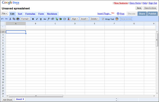
The Edit tab displays a toolbar full of editing options. From left to right, there are buttons for undo and redo; cut, copy, and paste; number formatting; text formatting (bold, italic, and so on); cell alignment; and inserting and deleting cells. There’s also a button to add a chart to your spreadsheet, based on selected data.
The Sort tab displays an abbreviated toolbar of sort-related options. You can sort the selected cells in normal or inverse order, or opt to freeze the header rows for easier sorting.
The Formulas tab displays a Range Names button, which you can use to name a range of cells. There are also links to insert some of the most common functions (Sum, Count, Average, Min, Max, and Product), as well as a More link that displays all available functions.
The Form tab provides quick access to tools for creating, sending, and embedding spreadsheets, as well as creating forms. Data entered via these forms is automatically inserted into the underlying spreadsheet.
The Revisions tab displays a pull-down list of the various versions of the current file. You can also use the Older and Newer buttons to switch to a different version.
Outside the tabs are a handful of common buttons. For example, the File button lets you open, save, and otherwise manage your spreadsheet files. Likewise, the Print button lets you print your spreadsheet, and the Save button lets you save your work.
Like Excel, Google Spreadsheets lets you work with multiple sheets within a single spreadsheet file. Unlike Excel, which always starts with three sheets per spreadsheet, Google defaults to a single sheet. You can then add sheets to this first sheet.
To add a new sheet to your spreadsheet, all you have to do is click the Add Sheet button at the bottom of the main spreadsheet window. To switch to a different sheet, just click its link.
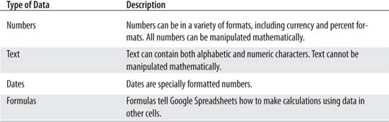
Google Spreadsheets lets you enter four different types of data, as detailed in Table 20.1.
Entering data is as simple as selecting a particular cell and typing input from the keyboard. Just move the cursor to the desired cell, using either the mouse or the keyboard arrow keys, and begin typing.
This approach works for all types of data, with the exception of formulas. Entering a formula is almost as simple, except that you must enter an equals sign (=) first. Just go to the cell, press the = key on the keyboard, and then enter the formula.
As to how the individual data is formatted—that is, how Google Spreadsheets interprets numbers and letters—it depends on what type of data you enter:
-
If you typed only numbers, the data is formatted as a number (with no commas or dollar signs).
-
If you typed a number with a dollar sign in front of it, the data is formatted as currency.
-
If you typed any alphabetic characters, the data is formatted as text.
-
If you typed numbers separated by the – or / character (such as 12–31 or 1/2/09), the data is formatted as a date.
-
If you typed numbers separated by the : character (such as 2:13), the data is formatted as a time.
Editing existing data in a cell is a fairly simple exercise; you actually edit within the cell. Just move the cursor to the desired cell and press the F2 key; this opens the cell for editing. Move the cursor to the data point within the cell you want to edit, and then use the Delete and Backspace keys to delete characters, or use any other key to insert characters. Press Enter when you are finished editing, and your changes are accepted into the selected cell.
Tip
If you accidentally delete data you want to keep, don’t panic! Google Spreadsheets includes an Undo option that lets you unwind your last command. All you have to do is click the Undo button at the top right of the workspace. Presto! You’ve undone your last delete, and your data is back where it belongs.
To insert a new row or column into a spreadsheet, start by positioning the cursor in the row or column where you want to insert a new row or column. Click the Insert button, and select whether you want to insert a row (above or below) or a column (to the right or left). Google Spreadsheets does the rest.
You can also delete entire rows and columns, or clear the contents of individual cells. To delete a row or column, position the cursor in that row or column, click the Delete button, and select whether you want to delete the row or column. To clear the contents of a cell, you do the same thing but select Clear Selection when you click the Delete button.
When you reference data within a spreadsheet, you can reference individual cells or you can reference a range of cells. When you reference more than one contiguous cell, that’s called a range. You typically use ranges with specific functions, such as SUM (which totals a range of cells) or AVERAGE (which calculates the average value of a range of cells).
A range reference is expressed by listing the first and last cells in the range, separated by a colon (:). For example, the range that starts with cell A1 and ends with cell A9 is written like this:
A1:A9
You can select a range with either the mouse or keyboard. Using the mouse, you can simply click and drag the cursor to select all the cells in the range. Using the keyboard, position the cursor in the first cell in the range, hold down the Shift key, and then use the cursor keys to expand the range in the appropriate direction.
Finally, you can use a combination of mouse and keyboard to select a range. Use either the mouse or keyboard to select the first cell in the range. Then hold down the Shift key and click the mouse in the last cell in the range. All the cells between the two cells are automatically selected.
Often, you want your data to appear in a sorted order. You might want to sort your data by date, for example, or by quantity or dollar value. Fortunately, Google Spreadsheets lets you sort your data either alphabetically or numerically, in either ascending or descending order.
Tip
The A>Z and Z>A sorts don’t just sort by letter; they also sort by number. An A>Z sort arranges numeric data from smallest to largest; a Z>A sort arranges numeric data from largest to smallest.
Sorting data in Google Spreadsheets is a two-step operation. First you have to “freeze” the header row(s) of your spreadsheet, and then you identify the column by which you want to sort. Google then orders all the “unfrozen” (non-header) rows of your spreadsheet in whichever order (ascending or descending) you specified.
Start by selecting the Sort tab, and then click the Freeze Rows button and select how many rows you want to include as the spreadsheet’s header. Next, identify which column you want to sort by, and move the cursor to any cell within that column. Finally, to sort in ascending order, click the A>Z button; to sort in descending order, click the Z>A button.
Let’s face it—a basic Google spreadsheet looks pretty plain. Fortunately, you can spruce it up by changing font size, family, and color, and by changing the background color of individual cells. All you have to do is select the cell(s) you want to format, and then use the formatting options on the Edit tab toolbar.
Note
Although you can change text attributes for an entire cell or range of cells, Google Spreadsheets doesn’t let you change attributes for selected characters within a cell.
You can also change how numbers are formatted within your spreadsheet. A number can be expressed as a whole number, as a percentage, as a fraction, as currency, as a date, and even exponentially. To apply a different number format, just select the cell or range, click the Format button (on the Edit tab), and then select a format.
After you’ve entered data into your spreadsheet, you need to work with those numbers to create other numbers. You do this as you would in the real world, by using common formulas to calculate your data by addition, subtraction, multiplication, and division. You can also used advanced formulas preprogrammed into Google Spreadsheets; these advanced formulas are called functions.
A formula can consist of numbers, mathematical operators, and the contents of other cells (referred to by the cell reference). You construct a formula from the following elements:
-
An equals sign (=); this is necessary at the start of each formula.
-
One or more specific numbers.
and/or
-
One or more cell references.
-
A mathematical operator (such as + or –); this is needed if your formula contains more than one cell reference or number.
For example, to add the contents of cells A1 and A2, you enter this formula:
=A1+A2
To multiply the contents of cell A1 by 10, you enter this formula:
=A1*10
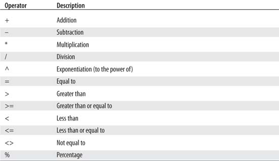
And so on. Table 20.2 shows the algebraic operators you can use within Google Spreadsheets formulas.
To enter a formula in a cell, move the cursor to the desired cell, type = to start the formula, and then enter the rest of the formula. Remember to refer to specific cells by the A1, B1, and so on cell reference. Press Enter to accept the formula or press Esc to reject the formula.
Tip
You can use the mouse to enter cell references into your formulas. Use the keyboard to enter the =, and then use the mouse to select the cell or range of cells to include. Use the keyboard again to enter any operators, and then use the mouse again to select additional cells. Press Enter to finish the formula.
When you’re finished entering a formula, you no longer see the formula within the cell; instead, you see the results of the formula. For example, if you entered the formula =1+2, you see the number 3 in the cell. To view the formula itself, just select the cell and then look in the reference area in the lower-right corner of the spreadsheet window.
A function is a type of formula built into Google Spreadsheets. You can use Google’s built-in functions instead of writing complex formulas in your spreadsheets; you can also include functions as part of your formulas.
Functions simplify the creation of complex formulas. For example, if you want to total the values of cells B4 through B7, you could enter the following formula:
=B4+B5+B6+B7
Or you could use the SUM function, which lets you total (sum) a column or row of numbers without having to type every cell into the formula. In this instance, the formula to total the cells B4 through B7 could be written using the SUM function, like this:
=sum(B4:B7)
This is much easier, don’t you think?
Google Spreadsheets uses most of the same functions as those used in Microsoft Excel. All Google functions use the following format:
=function(argument)
Replace function with the name of the function, and replace argument with a range reference. The argument always appears in parentheses.
You can enter a function into a formula either by typing the name of the function or by pasting the function into the formula from a list of functions displayed on the Formula tab. (You don’t have to be on the Formula tab to enter functions manually, however.)
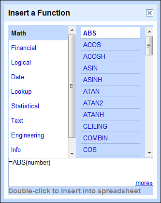
To use the Formula tab to enter formulas, move the cursor into the cell you want to hold the results of the function. Click the More link at the top right of the page and, when the Insert a Function dialog box appears, as shown in Figure 20.2, click the function you want to use. When you click the Close link, the function is pasted into the selected cell.
Google Spreadsheets also lets you chart your data. This functionality is relatively new; it wasn’t in the initial version of the application.
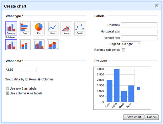
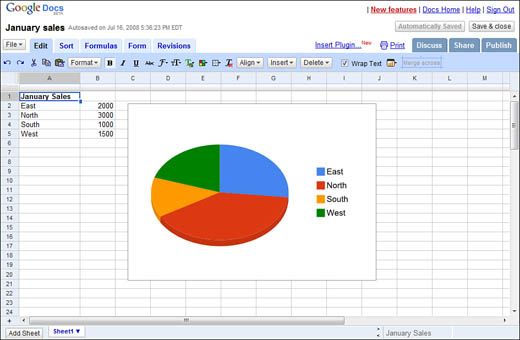
To create a chart, start by selecting the Edit tab, then select the cells that include the data you want to graph and click the Add button and select Chart. This displays the Create Chart dialog box, shown in Figure 20.3. You can create six types of charts—columns, bars, pie, lines, area, and scatter—and different subtypes within each major type. Select the type of chart you want, along with the subtype, enter a chart title, and select any other desired options (such as a chart legend). When the preview looks like you want it to, click the Save Chart button. The chart is created and added to the current spreadsheet, as shown in Figure 20.4.
When you’re finished creating your spreadsheet, you might want to print a hard copy. This is fairly easy to do. Just click the Print button on the selected spreadsheet page. When the Print dialog box appears, make sure that the correct printer is selected, and then click the Print button.
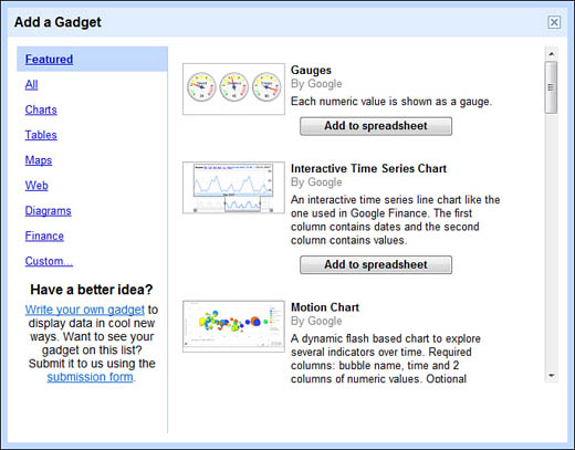
As noted earlier, Google Spreadsheets doesn’t have all the functionality you find in Microsoft Excel. You can increase the functionality, however, by adding various gadgets to your spreadsheets.
In the Google Spreadsheets world, a gadget is a plug-in that adds functionality to the basic application. Gadgets are created both by Google and by other users; you can also create your own gadgets if you’re so inclined. You can find gadgets that create more sophisticated chart types, add pivot table functionality, and the like. This is a great way for Google to make Google Spreadsheets better without having to alter the core application code.
To add a gadget to a spreadsheet, either click the Insert Plugin link or go to the Edit tab, click the Add button, and then select Gadget. This displays the Add a Gadget dialog box, shown in Figure 20.5. Select the type of gadget you want, and then click the Add to Spreadsheet button to add the gadget.
One of the key reasons to use Google Spreadsheets is the collaboration function. Because it’s a Web-based application, it’s relatively easy to share a spreadsheet with others—and to collaborate on a single spreadsheet as a group.
We covered Google Docs’ sharing and collaboration functions in depth in Chapter 19, “Using Google Docs.” Those functions work pretty much the same in Google Spreadsheets as they do in the word processing application. You find the sharing/collaboration functions on the Share tab and the publishing functions on the Publish tab.
You can also use Google Spreadsheets offline, thanks to Google Gears. This lets you access your spreadsheets even when you’re not connected to the Internet. Learn more about this functionality in Chapter 19 as well.