
Chapter 7. Essential Mathematics and the Geometry of 2-Space and 3-Space
7.1. Introduction
Unlike other chapters in this book, this one covers a great deal of material with which you may already be familiar in some form. The goals of this organization of the material are
• To have it all in one place, where you can easily refer to it
• To present it in a way that has a somewhat different approach from what you may have seen in the past, one that’s particularly useful for graphics
Much of the chapter will be easy reading; the material will look familiar. To be sure it really is familiar, we include a number of exercises in the chapter itself; you should work through these exercises to be certain you really are understanding what you’re reading. We assume that you’ve encountered some linear algebra, and are familiar with vectors, matrices, linear transformations, and notions like “basis” and “linear independence.”
One test, as you read this material, is to ask yourself, “Could I write code to implement this idea?” If the answer is no, you should spend more time understanding the concept. This is sufficiently important that we embody it in a principle, which one of us first heard expressed by Hale Trotter of Princeton in the 1970s.
![]() The Implementation Principle
The Implementation Principle
If you understand a mathematical process well enough, you can write a program that executes it.
We add to this the idea that often, writing such a program removes the necessity of understanding the details in the future: If you’ve done a good job, you can reuse your program.
7.2. Notation
We’ll use conventional mathematical notation, in which most variables appear in italics; vectors will be written in roman boldface (e.g., u), as will matrices. In general, vectors will be lowercase, matrices uppercase. When a variable has a subscript used for indexing, it’s italic, as in the i in ![]() . When a subscript or superscript is mnemomic, as in ρdh, the “directional hemispherical reflectance,” it’s in roman font.
. When a subscript or superscript is mnemomic, as in ρdh, the “directional hemispherical reflectance,” it’s in roman font.
Certain special sets have predefined names and are written in boldface font: R is the set of real numbers; C is the set of complex numbers; R+ (pronounced “R plus”) is the set of positive real numbers; and ![]() (pronounced “R plus zero”) is the set of non-negative reals.
(pronounced “R plus zero”) is the set of non-negative reals.
7.3. Sets
Sets are generally denoted by capital letters. The Cartesian product of the sets B and C is the set
1. This notation means “the set of all pairs (b, c) such that b is in B and c is in C.” That is, the colon is read “such that.”
which is pronounced “B cross C”; despite this, it is called a “Cartesian” product rather than a “cross product”; that term is reserved for the cross product of vectors discussed in Section 7.6.4.
The product R × R is denoted R2; higher order products are R3, R4, etc., with the n-fold product being Rn.
The closed interval [a, b] is the set of all real numbers between a and b, inclusive, that is,
If b < a, then the interval is empty; if b = a, the interval contains just the number b. We’ll also occasionally use intervals that contain just one of their endpoints (i.e., half-open intervals):
We also define the following two notational conventions:
7.4. Functions
The notion of a function is already familiar to you from both mathematics and programming. We’ll use a particular notation to express functions; an example is
The name of the function is f. Following the colon are two sets. The one to the left of the arrow is called the domain; the one to the right is called the codomain (some books use the term “range” for this; however, “range” is also used in a similar but different sense, leading to confusion). Following the second colon is a description of the rule for associating to an element of the domain, x, an element of the codomain.
This corresponds closely to the definition of a function in many programming languages, which tends to look like this:
1 double f(double x)
2 {
3 return x * x;
4 }
Once again, the function is named; the domain is explicitly defined (“x can be any double”), and the codomain is explicitly defined (“this function produces doubles”). The rule for associating the typical domain element, x, with the resultant value is given in the body of the function.
Mathematics allows somewhat subtler definitions than do most programming languages. For example, we can define
in mathematics, but most languages lack a data type which is a “non-negative real number.” The distinction between f and g is important, however: In the case of g the set of values produced by the function (i.e., the set {x2 : x ε R}) turns out to be the entire codomain, while in f it is a proper subset of the codomain. The function g is said to be surjective, while f is not. (Some books say that “g is onto.”).
If we define
we get yet a different function. The function h is not only surjective, it has another property: No two elements of the domain correspond to the same element of the codomain; that is, if h(a) = h(b), then a and b must be equal. Such a function is called injective.2 A function like h that’s both injective and surjective has an inverse, denoted h–1, a function that “undoes” what h does. The domain of h–1 is the codomain of h, and vice versa. In the case of our particular function, the inverse is
2. Some books use the term “one-one” or “one-to-one,” but others use the same term to mean both injective and surjective.
is an injective and surjective (or bijective) function, its inverse,
is the unique function satisfying
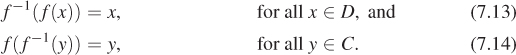
Figure 7.1 illustrates these three classes of functions.
Figure 7.1: Three different functions: (a) is surjective but not injective; (b) is injective but not surjective; and (c) is bijective.
Which of the following functions have inverses? Describe the inverses when they exist.
(a) The negation function N : R ![]() R : x
R : x ![]() –x.
–x.
(b) q1 : R ![]() R : x
R : x ![]() arctan(x).
arctan(x).
(c) q2 : R ![]() [–π/2, π/2]: x
[–π/2, π/2]: x ![]() arctan(x).
arctan(x).
In describing functions, we’ll always describe the domain, the codomain, and the rule that associates elements in the first to elements in the second. Sometimes these rules may involve cases, as in
just as the code for a function may involve an if statement. We will also always speak of functions by name (e.g., “the function f is continuous”) rather than saying “the function f (x) is continuous,” because f (x) denotes the value of the function at a point x; this value is usually not a function. If we need to include the variable name for some reason, we will write “the function x ![]() f(x) is continuous at x = 0, but not elsewhere,” for instance. This careful distinction becomes important when we discuss functions like the Fourier transform, F, which operate on functions, producing other functions. If we speak of “the function f
f(x) is continuous at x = 0, but not elsewhere,” for instance. This careful distinction becomes important when we discuss functions like the Fourier transform, F, which operate on functions, producing other functions. If we speak of “the function f ![]() F(f),” we are referring to the Fourier transform F; if we speak of “the function F(f),” we are referring to its value on a particular function f.
F(f),” we are referring to the Fourier transform F; if we speak of “the function F(f),” we are referring to its value on a particular function f.
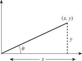
7.4.1. Inverse Tangent Functions
Mathematicians tend to define arctan, the inverse tangent function, from R to the open interval (–π/2, π/2). We’ll sometimes use this, and denote it u ![]() tan–1(u). A frequent use of the inverse tangent is to find the angle, θ, in the situation shown in Figure 7.2: We have the point with coordinates (x, y) and want to know θ. The usual answer is that when x > 0, it’s tan–1 (y/x), followed by several special cases for when x < 0, y > 0, or x < 0, y = 0, etc. These special cases have been built into a single function, atan2, which takes a pair of arguments, rather than a single one. It’s almost always used in the form θ = atan2(y, x), which does exactly what you would expect: It returns the angle between the x-axis and the ray from (0, 0) to (x, y). The returned angle is between –π and π. In the case where x and y are both zero, the returned value is zero. This makes atan2 discontinuous at the origin, as well as along the negative x-axis. On the negative x-axis, the IEEE version of atan2(y, x) returns either +π or –π depending on whether y = +0 or –0. The only tricky part is remembering that y comes first. You can remember this by knowing that if –π < θ < π, then
tan–1(u). A frequent use of the inverse tangent is to find the angle, θ, in the situation shown in Figure 7.2: We have the point with coordinates (x, y) and want to know θ. The usual answer is that when x > 0, it’s tan–1 (y/x), followed by several special cases for when x < 0, y > 0, or x < 0, y = 0, etc. These special cases have been built into a single function, atan2, which takes a pair of arguments, rather than a single one. It’s almost always used in the form θ = atan2(y, x), which does exactly what you would expect: It returns the angle between the x-axis and the ray from (0, 0) to (x, y). The returned angle is between –π and π. In the case where x and y are both zero, the returned value is zero. This makes atan2 discontinuous at the origin, as well as along the negative x-axis. On the negative x-axis, the IEEE version of atan2(y, x) returns either +π or –π depending on whether y = +0 or –0. The only tricky part is remembering that y comes first. You can remember this by knowing that if –π < θ < π, then
We’ll use atan2 not only in programs, but also in equations.
7.5. Coordinates
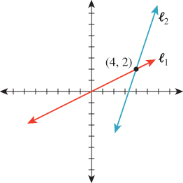
The Cartesian plane shown in Figure 7.3 is a model for Euclidean geometry: All of the axioms of geometry hold in the Cartesian plane, and we can use our geometric intuition to reason about it. A tabletop (or to be more accurate, an infinite tabletop) is also a model for Euclidean geometry. The difference between the two is that each point of the Cartesian plane has a pair of real numbers—its coordinates—associated to it. This lets us transform geometric statements like “the point P lies on the lines ![]() 1 and
1 and ![]() 2” to algebraic statements, like “the coordinates of the point P satisfy these two linear equations.” We can, of course, draw two perpendicular lines on the infinite tabletop, declare them to be the x- and y-axes, place equispaced tick marks along each, and use perpendicular projection onto these lines to define coordinates. But the choices we made—which line to call the x-axis, which to call the y-axis, what point to use as the origin, etc.—were arbitrary.3 It’s important to distinguish between the properties of a point or a line, and the properties of its coordinates; the underlying geometric properties don’t change when we change coordinate systems, while numerical properties of the coordinates do change. In Figure 7.4, you can see that the point P is on the line
2” to algebraic statements, like “the coordinates of the point P satisfy these two linear equations.” We can, of course, draw two perpendicular lines on the infinite tabletop, declare them to be the x- and y-axes, place equispaced tick marks along each, and use perpendicular projection onto these lines to define coordinates. But the choices we made—which line to call the x-axis, which to call the y-axis, what point to use as the origin, etc.—were arbitrary.3 It’s important to distinguish between the properties of a point or a line, and the properties of its coordinates; the underlying geometric properties don’t change when we change coordinate systems, while numerical properties of the coordinates do change. In Figure 7.4, you can see that the point P is on the line ![]() —that’s a geometric property; it’s true independent of any coordinate system.
—that’s a geometric property; it’s true independent of any coordinate system.
3. Indeed, Descartes did not even require that the two axes be perpendicular, although we now always choose them so.
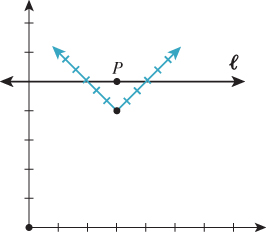
As an example of coordinate-dependent properties, the coordinates of P in the black coordinate system are (3, 5), while in the blue coordinate system they are (2, 2). Similarly, the equation of the line ![]() in the black coordinate system is y = 5, while in the blue coordinate system it’s x + y = 4. Thus, the point’s coordinates and the line’s equation are coordinate-dependent. But the fact that the point is on the line is coordinate-independent: Although P’s coordinates and
in the black coordinate system is y = 5, while in the blue coordinate system it’s x + y = 4. Thus, the point’s coordinates and the line’s equation are coordinate-dependent. But the fact that the point is on the line is coordinate-independent: Although P’s coordinates and ![]() ’s equation are different in the two systems, the black coordinates of P satisfy the black equation for
’s equation are different in the two systems, the black coordinates of P satisfy the black equation for ![]() , and similarly for the blue.
, and similarly for the blue.
From now on when we speak of “the coordinates of a point,” it will always be with respect to some coordinate system; much of the time the coordinate system will be obvious and we won’t mention it. For example, in R2, the set of ordered pairs of real numbers, the “standard” coordinates of the point (x, y) are just x and y.
7.6. Operations on Coordinates
Suppose (see Figure 7.5) we have the points P = (2, 5) and Q = (4, 1) in the plane, where the coordinates are with respect to the coordinate system drawn in horizontal and vertical black lines. If we average the coordinates of these points (averaging the x-coordinates and then averaging the y-coordinates) we get M = (3, 3), which turns out to be the midpoint of the segment between them. This is an interesting situation: The midpoint is defined purely geometrically, independent of coordinates. But we’ve got a formula, in coordinates, for computing it. Suppose we look at the coordinates of P and Q in the blue coordinate system, which is rotated 45° from the black one, and has its origin to the right and below, and average those: The coordinates are (2, 2) and (2, 4); the average is (2, 3). In the blue coordinate system, the point (2, 3) is exactly at the same location as the black coordinate system point (3, 3). In short, while the coordinate computations differ, the underlying geometric result is the same.
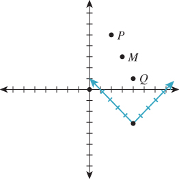
Figure 7.5: The coordinates of M in each coordinate system are the average of the coordinates of P and Q in that coordinate system; thus, the geometric operation of finding the midpoint of a segment corresponds to the algebraic operation of averaging coordinates, independent of what coordinate system we use.
Contrast this with the operation “divide the coordinates of a point by two” (Figure 7.6). Under this operation, the point P with black-line coordinates (2, 5) becomes the point P′ with coordinates (1, 2. 5). But if we apply the same operation in blue-line coordinates, where P has coordinates (4, 7), the new blue-line coordinates are (2, 3. 5), and the point P″ corresponding to those coordinates is far from P′. What’s the difference between the averaging and the divide-by-two operations? Why does “averaging coordinates” give the same result in any two coordinate systems, while “dividing coordinates by two” gives different ones? We’ll answer this in greater detail in Section 7.6.4. For now, let’s just examine the distinction algebraically: Let’s write down the average of the coordinates of points (x1, y1) and (x2, y2). It’s just

Figure 7.6: The operation “divide the coordinates of a point by two” produces different results (P′ and P″) in the two coordinate systems—this simple algebraic operation is not independent of the coordinate system, so it doesn’t correspond to any geometric operation.
If we agree to temporarily define a “multiplication” of a point’s coordinates by a number with the rule
and addition of points by
then this averaging can be written
while the “dividing coordinates by two” operation can be written
The key difference, it turns out, is that the first operation involves summing up terms where the coefficients sum to one (because ![]() ), while the second does not. A combination where the coefficients sum to one is called an affine combination of the points, and it is combinations like these that are invariant when we change coordinate systems. (You should try a few others to convince yourself of this.)
), while the second does not. A combination where the coefficients sum to one is called an affine combination of the points, and it is combinations like these that are invariant when we change coordinate systems. (You should try a few others to convince yourself of this.)
Since affine combinations have the property of being “geometrically meaningful,” we’ll now examine them more closely. Suppose that instead of averaging, we took a ![]() combination of the points, that is, we computed (for the points P and Q in Figure 7.5)
combination of the points, that is, we computed (for the points P and Q in Figure 7.5)
We’d get the point ![]() , which also lies on the line between P and Q, but is closer to Q. In fact, we can compute
, which also lies on the line between P and Q, but is closer to Q. In fact, we can compute
for any number α: With α = 1 we get Q; with α = 0 we get P; with α = ![]() we get M; and with any value of α between 0 and 1 we get points on the line segment between P and Q.
we get M; and with any value of α between 0 and 1 we get points on the line segment between P and Q.
What happens when we consider values of α that are less than 0? Those correspond to points on the line beyond P; similarly, ones with α > 1 are beyond Q. In summary:
With this in mind, we can define a function
The image of this function is the line between P and Q; if we restrict the domain to the interval [0, 1], then the image is the line segment between P and Q. We call this the parametric form of the line between P and Q, where the argument t is the parameter. (In Section 7.6.4 we’ll justify this particular use of the multiply-by-scalars-and-add operation applied to points.)
We discussed that certain coordinate constructions are invariant under changes in coordinate systems. If two people place coordinate systems on the same tabletop and compute lengths, angles, and areas, will they always get the same results? In other words, are lengths, angles, and areas invariant under changes of coordinates? If not, can you think of particular conditions on the coordinate systems under which these are invariant? Note: The length of the segment from (x1, y1) to (x2, y2) in a Cartesian coordinate system is defined to be ![]() ; you’ll need to figure out similar definitions of angle and area to answer this question.
; you’ll need to figure out similar definitions of angle and area to answer this question.
7.6.1. Vectors
We’ll return to lines presently; before we do so, however, we’ll codify some of the ideas above by relating them to vectors. The term “vector” gets used in many fields to mean many things. For now, we’ll content ourselves with one particular type of vector, a coordinate vector, which is simply a list of real numbers. An n-vector is a list of n numbers; we’ll write these between square brackets, organized vertically:
for example, is a 3-vector. A generalization of this notion is that of matrices, which are doubly indexed lists of real numbers, named by the number of rows and the number of columns. Thus,
is a 3 by 2 (often written 3 × 2) matrix. Entries of the matrix are indicated by subscripts, with the row index first; if A is a matrix, then aij denotes the entry in row i, column j. An n-vector can be considered an n × 1 matrix. An important operation on matrices is transposition: An n × k matrix A becomes a k × n matrix whose ij entry is the ji entry of A. Thus, the transpose of the matrix above is
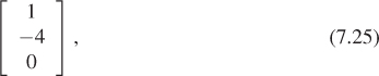
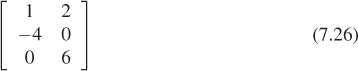
The transpose of the matrix A is written AT. Because horizontal lists fit typography better than do vertical ones, we’ll often describe a vector by its transpose. Thus, if v is the vector above, we might write “Let v = [1 –4 0]T ...” as a way of introducing it into the discussion.
7.6.1.1. Indexing Vectors and Arrays
In mathematics, vectors and matrices use one-based indexing: If v is a vector, its first element is written v1, its second v2, etc. If M is a matrix, the element in row i and column j is denoted mij; when i and j are particular integers, these are sometimes separated by commas, as in m1,2.
7.6.1.2. Certain Special Vectors
In R2, any vector [a b]T can be expressed in the form
the two vectors on the right are called e1 and e2. In R3, we have a similar set of vectors; the names are reused:
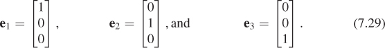
In general, in Rn, the name ei refers to a vector whose entries are zeroes, except the ith, which is 1.
The vector whose entries are all zero (in any dimension) is denoted 0; note the boldface font.
7.6.2. How to Think About Vectors
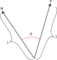
It’s common for students to say, “A vector is an arrow.” So, when asked if the vectors v and w in Figure 7.7 are the same, they answer “yes,” although the two arrows, being in different places, are clearly different. A better way to think of a vector is as a displacement—it represents an amount by which you must move to get from one place to another. For example, to get from the point (3, 1) to the point (5, 0), you must move by 2 in the x-direction and by –1 in the y-direction. This displacement is represented by the vector [2 –1]T. It’s exactly the same as the displacement needed to move from (4, 1) to (6, 0). With this interpretation, addition of vectors makes sense: You add corresponding terms. And multiplication by a constant is similarly defined by multiplying each entry by that constant, thus increasing or decreasing the displacement.
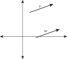
Figure 7.7: The arrows labeled v and w are often considered to be “the same,” even though they are clearly different entities. If we think of each of them as representing a displacement of the plane (i.e., a motion of all points of the plane up and to the right), then although the arrows themselves are distinct, they represent the same displacement.
If the word “displacement” is not satisfactory, you can also think of vectors as “differences between points,” that is, as a description of the amount you would have to move the first point to reach the second. The same pair of points, moved to a different location by a shift in x and y, correspond to the same vector, because the difference between them is unchanged.
7.6.3. Length of a Vector
The length (or norm) of the vector v, denoted ||v||, is the square root of the sum of the squares of the entries of v. If v = [1 2 3]T, then ![]() . This corresponds, when we think of v as a displacement, to the distance that we moved. A vector whose length is 1 is called a unit vector.
. This corresponds, when we think of v as a displacement, to the distance that we moved. A vector whose length is 1 is called a unit vector.
You can convert a nonzero vector v to a unit vector, which is called normalizing it, by dividing it by its length. We write
for this, with the letter “S” being chosen for “sphere,” since normalizing a vector in 3-space amounts to adjusting its length so that its tip lies on the unit sphere.
7.6.4. Vector Operations
We can add vectors and multiply a vector by a constant (called scalar multiplication); more generally, if we have several vectors v1, v2, ..., vn, and numbers c1, c2, ..., cn, we can form the linear combination
The set of all linear combinations of a single nonzero vector v is the line containing v (where here we are reverting temporarily to the notion of the vector v representing the endpoint of an arrow starting at the origin); the set of all linear combinations of two nonzero vectors v and w is, in general, the plane that contains both of them. One exception is when one vector is a multiple of the other, in which case the result is the line containing both.
Aside from addition and multiplication by a constant, there are two other operations on vectors that we’ll often use: dot product and cross product.
7.6.4.1. Cross Product
The cross product is usually defined for pairs of vectors in 3-space as follows:
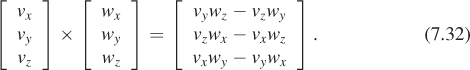
The cross product is anticommutative, that is, v × w = –w × v (the labeling and ordering of the subscripts was chosen to make this self-evident). It’s distributive over addition and scalar multiplication, but not associative. One of the main uses of the cross product is that
where θ is the angle between v and w. That means that half the length of the cross product is the area of the triangle with vertices (0, 0, 0), (vx, vy, vz), and (wx, wy, wz).
The cross product can be generalized to dimension n; in dimension n, it’s a product of n – 1 vectors (which explains why the n = 3 case is the most often used). Aside from dimension 3, our most frequent use will be in dimension 2, where it’s a “product” of one vector. The cross product of the vector is
This cross product has an important property: Going from v to ×v involves a rotation by 90° in the same direction as the rotation that takes the positive x-axis to the positive y-axis. Because of this, it’s sometimes also denoted by v⊥.
In the same way, going from v to w to v × w describes a right-handed coordinate system, one in which placing your right-hand pinkie on the first vector and curling it toward the second makes your thumb point in the direction of the third (see Figure 7.8). In general, in n dimensions, the cross product z of n – 1 vectors v1, ..., vn–1 lies in a line perpendicular to the subspace containing v1, ..., vn–1. The length of z is (n – 1)! times the (n – 1)-dimensional volume of the pyramid-like shape whose vertices are the origin and the endpoints of vi. Assuming this volume is nonzero, z is oriented so that v1, v2, ..., vn–1, z is “positively oriented” in analogy with the right-hand rule in three dimensions.
7.6.4.2. Dot Product
From linear algebra, you’re familiar with the dot product of two n-vectors v and w, defined by
This is sometimes denoted ![]() v, w
v, w![]() ; in this form, it’s usually called the inner product. The dot product is used for measuring angles. If v and w are unit vectors, then
; in this form, it’s usually called the inner product. The dot product is used for measuring angles. If v and w are unit vectors, then
where θ is the angle between the vectors (Figure 7.9). This is most often used in the form
which gives the angle between any two nonzero vectors, expressed as a number between 0 and π, inclusive.
Fix the vector w ![]() R2 for a moment. The function
R2 for a moment. The function
tells “how much v is like w” in the sense that as v ranges over all displacements of a fixed length—say, length 1—this function is most positive when v is parallel to w, most negative when it’s a displacement in the direction opposite w, and zero for displacements that are in directions perpendicular to w.
The dot product is central to much of linear algebra; a surprising number of computations and simplifications can be done by working with vectors and their dot products rather than with their coordinates. This often leads to insight into the underlying operations.
7.6.4.3. The Projection of w on v
As an example of the use of dot products, suppose we want to write the displacement w as a sum,
where v′ is parallel to v and u is perpendicular to it (see Figure 7.10). How can we find v′? First, we know it’s a multiple sv of v; all we need to find is s. Consider the dot product of v with both sides of Equation 7.39:
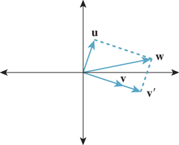
Figure 7.10: Decomposing a displacement w as a sum of two displacements, one parallel to a given vector v and one perpendicular to v.
The projection is therefore
And u is just
When v is a unit vector, the expression for v′ simplifies to
7.6.4.4. Operations on Points and Vectors
With the notion of a vector as a difference between points, or as a displacement, we can write down a number of operations.
• The difference between points P and Q, denoted by P – Q, is a vector.
• The sum of a point P and a vector v is another point. In particular, P + (Q – P) = Q.
• The sum or difference of vectors is defined by elementwise addition or subtraction.
• The sum of two points isn’t defined at all.
Thus, although for both points and vectors in the plane we represent each with a pair of real numbers, we use the typographical convention that points are denoted by tuples like (3, 6), while vectors are denoted by 2 × 1 matrices in square brackets. In software (see Chapter 12), it’s helpful to also make vectors and points have different types. In an object-oriented language, we would define the classes Point and Vector. The first would contain an AddToVector operation, but not an AddToPoint operation; the second would have both (with results of types Vector and Point, respectively). Such a distinction allows the compiler to save us from mistakes in our mathematical treatment of points and vectors.
If we, for a moment, use E2 to denote the set of points, but R2 to denote vectors, then we have defined
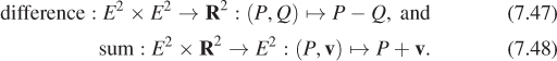
(Note that E2 × E2 is the Cartesian product of E2 with itself, i.e., the set of all pairs of points.) These definitions generalize in a natural way to Rn and En. In general, using these operations, we can define an affine combination of points. Even though we said we could not add points, we saw earlier that computing the midpoint between P and Q could be expressed nicely if we allowed ourselves to write things like
We’ll now make sense of that. The expression
which we call an affine combination of P and Q, will be defined only when α + β = 1. If we pretend for a moment that all sorts of arithmetic on points is well defined, then we can add βP and subtract it, to get
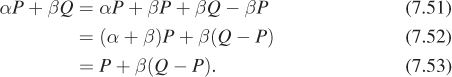
With this cavalier bit of algebra as motivation, we define αP + βQ to mean
which makes sense because Q – P is a vector, and hence β(Q – P) is as well; this vector can be added to the point P to get a new point. This definition naturally generalizes to an affine combination of more than two points; for instance, αP + βQ + γR, where α + β + γ = 1,
We’ll frequently encounter such affine combinations of points, especially when we discuss splines in Chapter 22. Mann et al. [MLD97] make a case for treating all of graphics in terms of such “affine geometry,” and abandoning coordinates to the degree possible. In fact, it makes sense to include an AffineCombination method for Points, to avoid errors or code that can be baffling. Listing 7.1 shows a possible implementation.
Listing 7.1: Code in C# for creating an affine combination of points, with a special case for two points.
1 public Point AffineCombination(double[] weights, Point[] Points)
2 {
3 Debug.assert(weights.length == Points.length);
4 Debug.assert(sum of weights == 1.0);
5 Debug.assert(weights.length > 0);
6
7 Point Q = Points[0];
8 for (int i = 1; i < weights.length; i++) {
9 Q = Q + weights[i]* (Points[i] - Points[0]);
10 }
11 return Q;
12 }
13
14 public Point AffineCombination(Point P, double wP,
15 Point Q, double wQ)
16 {
17 Debug.assert( (wP + wQ) == 1.0);
18
19 Point R = P;
20 R = R + wQ * (Q - P);
21 return R;
22 }
7.6.5. Matrix Multiplication
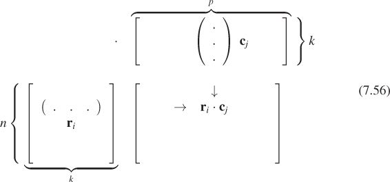
The product of two matrices A and B is defined only when the number of columns of A matches the number of rows of B. If A is n × k and B is k × p, then the product AB is an n × p matrix. If we let the ith row of A be the transpose of the vector ri, and the jth column of B be the vector ci, then the ijth entry of AB is just ri · cj. The following picture may help you remember this:
Thus, we see that the dot product of the vectors v and w is just the matrix product vTw:
This leads to an interpretation of the product of the matrix A (with rows ai) and a vector v: If w = Av, then the ith entry of w tells “how much v looks like ![]() ” (in the sense described when we discussed Equation 7.38).
” (in the sense described when we discussed Equation 7.38).
There’s another equally useful interpretation of Av. If we let bi denote the columns of A, then
that is, the product of A with v is a linear combination of the columns of A.
One particularly useful consequence of the definition of Av is that if we want to multiply A by several vectors v1, v2, ..., vk, we can express this product by concatenating the vectors vi into a matrix V whose columns are v1, v2, etc.; the product
is then a matrix W whose ith column is Avi. This is no more computationally efficient than multiplying A by each individual vector. The key application of this idea is when we have one set of vectors v1, v2, ..., vk and a second set of vectors w1, w2, ..., wk, and we wish to find a matrix with Avi = wi for i = 1, ..., k, that is, we wish to have
Often it’s impossible to achieve exact equality, but it will turn out that we can find the “best” such matrix A by straightforward operations on the matrices V and W, but we’ll wait to present the main ideas in context in Section 10.3.9.
In general, matrix multiplication is not commutative: AB ≠ BA.
(a) If A is a 2 × 3 matrix and B is a 3 × 1 matrix, show that AB makes sense, but BA does not.
(b) Let A = [1 2 3]T and B = [0 1 1]. Compute both AB and BA.
7.6.6. Other Kinds of Vectors
![]() The spaces R2 and R3 that we’ve been discussing, and Rn in general, have certain properties. There’s a notion of addition (which is commutative and associative), and of scalar multiplication (again associative, and distributive over addition). There’s also a zero vector with the property that 0 + v = v + 0 = v for any vector v. And there are additive inverses: Given a vector v, we can always find another vector w with w + v = 0. These properties, taken together, make Rn a vector space. There are a few other vector spaces we’ll encounter in graphics; some of these will arise in our discussion of images, others in our discussion of splines, and still others in our discussion of rendering. Most have a common form: They are spaces whose elements are all functions.
The spaces R2 and R3 that we’ve been discussing, and Rn in general, have certain properties. There’s a notion of addition (which is commutative and associative), and of scalar multiplication (again associative, and distributive over addition). There’s also a zero vector with the property that 0 + v = v + 0 = v for any vector v. And there are additive inverses: Given a vector v, we can always find another vector w with w + v = 0. These properties, taken together, make Rn a vector space. There are a few other vector spaces we’ll encounter in graphics; some of these will arise in our discussion of images, others in our discussion of splines, and still others in our discussion of rendering. Most have a common form: They are spaces whose elements are all functions.
Recall that, if we had a vector w ε R2, we built a function
This is a linear function on R2, and in fact, any linear function from R2 to R has this particular form.
Let f : R2 ![]() R be a linear function. Let a = f (e1), b = f (e2), and w = [a b]T. Show that for any vector v, we have f (v) = φw(v). You’ll need to use the fact that f is linear.
R be a linear function. Let a = f (e1), b = f (e2), and w = [a b]T. Show that for any vector v, we have f (v) = φw(v). You’ll need to use the fact that f is linear.
The collection of all such functions, that is,
forms a vector space: The sum of any two linear functions is again linear; the zero element of the vector space is φ0; and the additive inverse of φw is φ–w. Scalar multiplication deserves a brief comment. What does it mean to multiply a function from R2 to R by, say, 11? If f is such a function, then g = 11f is the function defined by
that is, one multiplies the output of f by 11.
This space of linear functions from R2 to R is called the dual space of R2, and its elements are sometimes called dual vectors or covectors. This same idea generalizes to R3 or even Rn. There’s an obvious correspondence between elements of R2 and elements of R2*, namely we can associate the vector w with the covector φw. So why not just call them “the same”? It will turn out that treating them distinctly has substantial advantages; in particular, we’ll see that when we transform all the elements of a vector space by some operation like rotation, or stretching the y-axis, the covectors transform differently in general.
In coordinate form, if w = [a b]T, then the function φw can be written
Some books therefore identify covectors with row vectors, and ordinary vectors with column vectors.
Note that in designing software, just as it made sense to distinguish Point and Vector, it makes sense to have a CoVector class as well.
Covectors are particularly useful in representing triangle normals (the normal to a triangle is a nonzero vector perpendicular to the plane of the triangle, and is used in computing things like how brightly the triangle is lit by light coming in a certain direction). Although people often talk about normal vectors, such vectors are almost always used as covectors. To be precise, when we have a vector n normal to a triangle, we will almost never add n to another vector or a point, but we’ll often use it in expressions like n · ![]() (where
(where ![]() might be, for instance, the direction that light is arriving from). Thus, it’s really the covector
might be, for instance, the direction that light is arriving from). Thus, it’s really the covector
that’s of interest.
7.6.7. Implicit Lines
We’ve already encountered the parametric form of a line (Equation 7.24). There’s another way to describe the line between P and Q: Instead of writing a function t ![]() γ(t) whose value at each real number t is a point of the line, we can write a different kind of function—one that tells, for each point (x, y) of R2, whether the point (x, y) is on the line. Such a function is said to define the line implicitly rather than parametrically. Such implicit descriptions are frequently useful; we’ll see shortly that computing the intersection of two parametrically described lines is more difficult than computing the intersection of a parametrically defined line and an implicitly defined one. Since the operation of intersecting lines (or rays) with objects is one that arises frequently in graphics (we’re very interested in where light, which travels in rays, hits objects in a scene!), we’ll examine such implicit descriptions more fully.
γ(t) whose value at each real number t is a point of the line, we can write a different kind of function—one that tells, for each point (x, y) of R2, whether the point (x, y) is on the line. Such a function is said to define the line implicitly rather than parametrically. Such implicit descriptions are frequently useful; we’ll see shortly that computing the intersection of two parametrically described lines is more difficult than computing the intersection of a parametrically defined line and an implicitly defined one. Since the operation of intersecting lines (or rays) with objects is one that arises frequently in graphics (we’re very interested in where light, which travels in rays, hits objects in a scene!), we’ll examine such implicit descriptions more fully.
If F : R2 ![]() R is a function, then for each c, we can define the set
R is a function, then for each c, we can define the set
which is called the level set for F at c. As an example, consider an ordinary weather map. To each point (x, y) on the map there’s an associated temperature T(x, y). The set of all points where the temperature is 80°F is a level set, as are the sets where the temperature is 70°F, 60°F, etc. These sets are typically drawn as curves on the map; each of them is a level set for the temperature function. Similarly, a contour map like the one in Figure 7.11 typically has contour lines for various heights—these curves represent the level sets of the height function. In graphics, we often build a function F whose level set for c = 0 constitutes some shape. This set is called the zero set of F.

Can two temperature-contour curves on a weather map ever cross? Why or why not?
7.6.8. An Implicit Description of a Line in a Plane
How can we find a function F whose value, on points of the line containing two distinct points P and Q, is zero, but whose value elsewhere is nonzero, that is, how can we find an implicit description of the line? Ponder that question briefly, then read on.
First,4 let n = ×(Q – P) = (Q – P)⊥; then the vector n is perpendicular to the line (see Figure 7.12). A nonzero vector with this property is said to be a normal vector or simply a normal to the line.
4. Note that we’re using the 2D cross product defined in Equation 7.34 here.
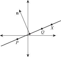
Figure 7.12: The vector n = (Q – P)⊥ is perpendicular to the line through P and Q. A typical point X of this line has the property that (X – P) is also perpendicular to n. Indeed, a point X is on the line if and only if (X – P) · n = 0.
The vector n is called a normal rather than the normal; show that this is justified by explaining why 2n and –n are also normals to the line.
If X is a point of the line, then the vector X – P points along the line, and so is also perpendicular to n. If X is not on the line, then X – P does not point along the line, and hence is not perpendicular to n. Thus,
completely characterizes points X that lie on the line. We can therefore define
which serves as an implicit description of the line. We’ll call this the standard implicit form for a line.
Our discussion assumes that P and Q are distinct. What set does the function F implicitly define if P and Q are identical?
As a concrete example, if P = (1, 0) and Q = (3, 4), then ![]() and
and ![]() . Letting X have coordinates (x, y), we have
. Letting X have coordinates (x, y), we have
as the implicit form of our line; expressed in coordinates, this says
or
which is the familiar Ax + By + C = 0 form for defining a line.
Both the implicit and parametric descriptions of lines generalize to three dimensions: Given two points in 3-space, the parametric form of Equations 7.28 given above will determine a line between them. The implicit form (i.e., (X – P) · n = 0) determines a plane passing through P and perpendicular to the vector n; to determine a single line, we must take two such plane equations with two nonparallel normal vectors.
7.6.9. What About y = mx + b?
In graphics we generally avoid the “slope-intercept” formulation of lines (an equation of the form y = mx + b; m is called the slope and the point (0, b) is the y-intercept, i.e., the point where the line meets the y-axis), because we cannot use it to express vertical lines; the “two-point” implicit and parametric forms above are far more general, and formulas involving them generally don’t need special-case handling.
7.7. Intersections of Lines
We now have two forms for describing lines in the plane: implicit and parametric. (The parametric form extends to lines in Rn.) With the help of the exercises, you can easily convert between them. If we have two lines whose intersection we need to compute, we could do an implicit-implicit, parametric-parametric, or parametric-implicit computation. The implicit-implicit version is messy enough that it’s better to convert one line to parametric form and use the implicit-parametric intersection approach. We’ll begin by computing the intersection of two lines in parametric form, mostly so that you see the benefit of the later implicit-parametric form. In general, we find that intersections between implicit and parametric forms tend to produce the simplest algebra.
7.7.1. Parametric-Parametric Line Intersection
Suppose we have two lines in parametric form, that is, two functions
whose images are (respectively) the line AB and the line CD (see Figure 7.13). We’d like to find the point P where these lines intersect. That point will lie on the line determined by γ, that is, it will be γ(t0) for some real number t0; similarly, it’ll be η(s0) for some real number s0. Equating these gives
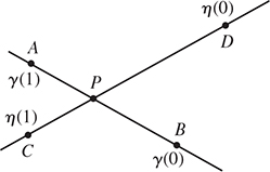
Figure 7.13: The lines AB and CD are the images of the parametric functions γ and η; they intersect at the unknown point P.
which can also be written
which is a nice form because it involves only vectors (i.e., differences between points).
If we write out Equation 7.74 in terms of the known coordinates of the points A, B, C, and D, we get two equations in the two unknowns s0 and t0 and can solve for them. We can then compute P by computing either t0A + (1 – t0)B or s0C + (1 – s0)D.
An alternative, and preferable, approach is to use the vector form shown in Equation 7.75. Letting v = A – B and u = C – D, we have
Taking the dot product of both sides with × v, we get
where the simplification arises because × v is perpendicular to v, so their dot product is zero. The last trick—eliminating a term from an equation by taking the dot product of both sides with a vector orthogonal to that term—is often useful.
7.7.2. Parametric-Implicit Line Intersection
Now suppose we’re given a parametric form for one line and an implicit form for a second line. How can we compute their intersection? We need to find the value t0 of t with the property that
is on the line defined by ![]() = {X : (X – S) · n = 0}.
= {X : (X – S) · n = 0}.
For this to be true, we need that
that is
Once again the vector form becomes useful as we simplify:
Writing u = Q – P and v = P – S, we have
Plugging this into the formula for γ(t0) yields the xy-coordinates of the intersection point T.
Carry out this final computation to find the coordinates of T. Try to do all your computations using dot products and vector operations rather than explicit coordinate computations.
Note that this computation gives us two things. It tells us where along the line determined by γ the intersection lies, by giving us t0; if t0 is between 0 and 1, for instance, we know that the intersection lies between P and Q. It also tells us the actual coordinates of the intersection point (x0, y0), that is, it provides an explicit point on the line that’s determined implicitly by Ax + By + C = 0. If we only care about intersections between P and Q, but find t0 is not between 0 and 1, we can avoid the second part of the computation.
7.8. Intersections, More Generally
In talking about intersections of lines, we’ve advocated the use of vectors and inner products. There are several advantages to this approach.
• Rather than writing out everything two (in two dimensions) or three (in three dimensions) times, once per coordinate, we write things just once, reducing the chance of error.
• Frequently the vector form of a computation generalizes naturally to n dimensions, while the generalization of the coordinate form may not be obvious (a nice example is the decomposition of a vector into a part parallel to a given vector u and a part that’s perpendicular to u; our formula works in 2-space, 3-space, 4-space, etc.).
• Our programs become easier to read and debug when we write less code. Programs written to reflect the vector description of computations are usually simpler.
We’ll consider two more examples of the vector form of computation of intersections: the intersection of a ray with a plane and with a sphere.
7.8.1. Ray-Plane Intersection
Let’s intersect a ray, given by its starting point P and direction vector d (so that a typical ray point is P + td, with t ≥ 0), with a plane, specified by a point Q of the plane and a normal vector n. A point X of the plane therefore has the property that
which generalizes the standard implicit form of a line in R2.
We seek a value, t ≥ 0, with the property that the point P + td is on the plane, for this point will be on both the plane and the ray, that is, at their intersection. Let’s proceed by assuming that such an intersection point exists and is unique; we’ll return to this assumption shortly.
For P + td to lie on the plane, it must satisfy
We can now simplify this considerably and solve for t as follows:
The reader will notice that this is essentially the same computation we did in Equation 7.87 earlier; once again, the vector form generalizes nicely.
In the algebra shown above, why did we not write P · n + td · n – Q · n = 0 as a simplification of the first equation?
Knowing t, we can now compute the intersection point P + td. Two small concerns remain:
• The possibility of division by zero in the expression for t
• The assumption that an intersection exists and is unique
These two concerns, it turns out, are identical! If d · n = 0, then the ray is parallel to the plane; that means it’s either contained in the plane (in which case there are infinitely many intersections) or disjoint from the plane, in which case there are none. In the first case, both the numerator and denominator are zero; in the second, only the denominator is.
What happens if we solve for t and find that it’s negative? That can happen if either the numerator or denominator is negative, and the other is positive. Describe each of these situations geometrically, as in “In the first case, P is on the positive side of the plane (i.e., the half-space into which n points), and . . .”
Let’s carry out the computation again, in this case with a plane specified by a point Q that lies in the plane, and two vectors, u and v, that lie in the plane and are linearly independent. Now, points in the plane can be written in the form
for some real numbers α and β. This version of the problem seems distinctly more difficult, in the sense that a solution will give us t, α, and β; that impression is partially correct, as we’ll see.
We want to find a value t ≥ 0 with the property that
for some values α and β. The first algebraic steps are similar. Move the points around so that a difference of points appears, and we’ll be working only with vectors:
Letting h = P – Q, we can see that now the problem is “Express the vector h as a linear combination of u, v, and d.” We could let M be the matrix whose columns are these three vectors, and the solution becomes
To implement this, we’d need to invert a 3 × 3 matrix, which is not difficult, but masks some of the essential features of the problem. First, it’s possible that M is not invertible, but even if this happens, there may be a solution to
(M is noninvertible when the ray is parallel to the plane; the solution exists when the ray lies in the plane, and indeed, in this case there are infinitely many solutions.) Second, the inversion must be redone for each new ray we want to intersect with the plane; that makes ray-plane intersection computationally intensive, which is bad.
An alternative is to say, “Let’s just compute n = u × v,” and use the previous solution; that’s an excellent choice, because the cross-product computation can be performed once, and stored for later reuse. The point here is that computing a ray intersection with the implicit form is computationally far easier than doing so with the parametric form of the plane.
7.8.2. Ray-Sphere Intersection
Once again, suppose we have a ray whose points are of the form P + td, with t ≥ 0. We want to compute its intersection with a sphere given by its center, Q, and its radius, r.
The implicit description of this sphere is that the point X is on the sphere if the distance from X to Q is exactly r; this is equivalent to the squared distance (which is almost always easier to work with) being r2, that is,
where we’ve used the fact that the squared length of a vector v is just v · v.
Now let’s ask, “Under what conditions on t is P + td on the sphere?” It must satisfy
Because the vector P – Q is going to come up a lot, we’ll give it a name, v; now we can simplify the expression above:
This last equation is a quadratic in t, which therefore has zero, one, or two real solutions.
Describe geometrically the conditions under which this equation will have zero, one, or two solutions, as in “If the ray doesn’t intersect the sphere, there will be no solutions; if ...”
Fortunately, it’s easy to tell whether a quadratic c + bt + at2 = 0 has zero, one, or two real solutions. The quadratic formula tells us that the solutions are
which are real if b2 – 4ac ≥ 0; the two solutions are identical precisely if the square root is zero, that is, if b2 = 4ac. In our case, this turns out to mean that there are two solutions if
and one solution if the two sides are equal.
Note that if we choose to represent our ray with a vector d that has unit length, this computation simplifies somewhat, since d · d = 1.
The examples above—line-line intersection, line-plane intersection, ray-sphere intersection—all serve to illustrate the following general principle.
![]() The Parametric/Implicit Duality Principle
The Parametric/Implicit Duality Principle
There’s a duality between parametric and implicit forms for shapes. In general, it’s easy to find an intersection between shapes where one is described implicitly and the other parametrically, and harder when either both are implicit or both are parametric.
7.9. Triangles
Triangles, which are familiar from geometry, are the building blocks of much of computer graphics. If a triangle has vertices A, B, and C, then a point of the form Q = (1 – t)A + tB, where 0 ≤ t ≤ 1 is on the edge between A and B (see Figure 7.14). Similarly, a point of the form R = (1 – s)Q + sC is on the line segment between Q and C if 0 ≤ s ≤ 1. Expanding this out, we get

Figure 7.14: The point Q = (1 – t) A + tB is on the edge between A and B (provided t ε [0, 1]), and (1 – s) Q + sC is on the line segment from Q to C (when s ε [0, 1]).
Equation 7.112 is worth examining carefully in several ways. First, we can define a function,
whose image is exactly the triangle ABC (see Figure 7.15). F sends the entire right edge (s = 1) of the square to the single point C. Vertical lines (s = constant) are sent to lines parallel to AB. Horizontal lines (t = constant) are sent to lines through C and a point of the edge AB. This parameterization of the triangle (the variables s and t are the parameters) is often used in graphics.
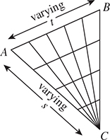
Figure 7.15: The function F : [0, 1] × [0, 1] ![]() R2 : (s, t)
R2 : (s, t) ![]() (1 – s)(1 – t)A + (1 – s)tB + sC, from the unit square to the triangle ABC, sends the entire s = 1 edge to the point C. All other lines in the square are sent to lines in the triangle as shown.
(1 – s)(1 – t)A + (1 – s)tB + sC, from the unit square to the triangle ABC, sends the entire s = 1 edge to the point C. All other lines in the square are sent to lines in the triangle as shown.
7.9.1. Barycentric Coordinates
Let’s also look at the coefficients in Equation 7.112: They are (1 – s)(1 – t), (1 – s)t, and s. It’s easy to see that for 0 ≤ s, t ≤ 1, all three are positive; summing them up we get
(This is good: Combinations of multiple points are only defined when the coefficients sum to one.) So we can say that the points of the triangle are of the form
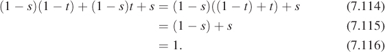
where α + β + γ = 1, and α, β, γ ≥ 0. Points where α = 0 lie on the edge BC; points where β = 0 lie on the edge AC; points where γ = 0 lie on the edge AB. If P = αA + βB + γC, then the numbers α, β, and γ are called the barycentric coordinates of P with respect to the triangle ABC.
(a) What are the barycentric coordinates of the midpoint of the edge AB in the triangle ABC? (b) What about the centroid?
Suppose A = (1, 0, 0), B = (0, 1, 0), and C = (0, 0, 1), and the point P of triangle ABC has barycentric coordinates α, β, and γ. What are the 3D coordinates of P?
Two other descriptions of the barycentric coordinates of a point in a triangle are often useful.
• In a nondegenerate triangle ABC, the A-coordinate of a point P is the perpendicular distance of P from the edge BC, scaled so that the A-coordinate of the point A is exactly one. There are two ways to see this. The first is to simply write everything out in terms of coordinates. The other is to realize that the “perpendicular distance” function and the “A-coordinate” function are both affine functions on the plane, and they agree at three points (A, B, and C), and this suffices to determine them uniquely.
• From the preceding description, it’s easy to see that the area of the triangle PCB, being half the product of the length of BC and the length of the perpendicular from P to BC, is proportional to that perpendicular length. So the A-coordinate of P is proportional to the area of triangle PBC. The proportionality constant is exactly the area of ABC, that is, the A-coordinate of P is
The same proof works for this case. In short, the point P provides a natural partition of the triangle ABC into three subtriangles; the fractions of the area of ABC represented by each of these triangles are the barycentric coordinates of P (Figure 7.16).
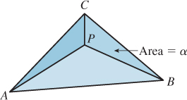
Figure 7.16: The point P divides triangle ABC into three smaller triangles, whose areas are fractions α, β, and γ of the whole; the barycentric coordinates of P are α, β, and γ, that is, P = αA + βB + γC.
7.9.2. Triangles in Space
The formulas given above—the parameterization of the triangle by a square, and the barycentric coordinates—don’t depend on the dimension. They work just as well when the points A, B, and C are in 3-space as in the plane! There is one aspect of a triangle in 3-space that’s different from the planar case: A triangle in 3-space is contained in a particular plane defined by an implicit equation of the form F(X) = (X – P) · n = 0. For P, we can use any of the three vertices of the triangle; for n, we can use the cross product
If the angle at B is very near zero or π, this computation can be numerically unstable (see Section 7.10.4).
With this in mind, let’s solve a frequently occurring problem: finding the intersection of a ray t ![]() P + td with a triangle ABC in 3-space. There are several cases. The intersection might occur where t < 0; the line containing the ray might not intersect the triangle at all; or the ray and the triangle might be in the same plane, and their intersection could be empty, a point, or a line segment. These last few cases have the property that a tiny numerical error—a slight change to one of the coordinates—can change the answer entirely. Such instabilities make the answers we compute almost useless. So, if the direction vector d is sufficiently close to perpendicular to the normal vector n, we’ll return a result of “UNSTABLE” rather than computing an intersection. Our strategy is to first find the parameter t at which the ray intersects the plane of the triangle, then find Q = P + td, the intersection point in the plane, and finally find the barycentric coordinates of Q, which in turn tell us whether Q is inside the triangle.
P + td with a triangle ABC in 3-space. There are several cases. The intersection might occur where t < 0; the line containing the ray might not intersect the triangle at all; or the ray and the triangle might be in the same plane, and their intersection could be empty, a point, or a line segment. These last few cases have the property that a tiny numerical error—a slight change to one of the coordinates—can change the answer entirely. Such instabilities make the answers we compute almost useless. So, if the direction vector d is sufficiently close to perpendicular to the normal vector n, we’ll return a result of “UNSTABLE” rather than computing an intersection. Our strategy is to first find the parameter t at which the ray intersects the plane of the triangle, then find Q = P + td, the intersection point in the plane, and finally find the barycentric coordinates of Q, which in turn tell us whether Q is inside the triangle.
For the most common situation—we’ll make many ray-intersect-triangle computations for a single triangle—it’s worth storing some additional data, per triangle, to speed the computation. We’ll precompute the normal vector, n, and two vectors AB⊥ and AC⊥, in the plane of ABC with the property that (a) AB⊥ is perpendicular to AB, and (C – A)· AB⊥ = 1, and similarly for AC⊥. If X is the point X = αA + βB + γC in the plane of ABC, then we can compute γ easily as γ = AB⊥ · (X – C), and a similar computation gives us β. Finally, we find α = 1 – (β + γ).
With these ideas in mind, Listing 7.2 shows the actual structure. If you consider any plane equation of the form f (X) = (X – A) · u = 0, then the value
is a linear function of t. For instance, if f is the equation of the plane of the triangle, we can solve for t to find the intersection of the ray with that plane. But suppose that f is the equation for the plane containing the edge AB and the normal vector n. Then f, when restricted to the triangle plane, is zero on the line AB, and nonzero on the point C (assuming the triangle is nondegenerate). That means that some multiple of f—namely X ![]() f (X)/f (C)—gives the barycentric coordinate at C. Now when we look at f (P + td), we can see how fast the C-coordinate of the projection of P + td into the triangle plane is changing. When we find the t-value at which the intersection occurs, we can therefore easily find the barycentric coordinate for the intersection point, as long as we know this plane equation.
f (X)/f (C)—gives the barycentric coordinate at C. Now when we look at f (P + td), we can see how fast the C-coordinate of the projection of P + td into the triangle plane is changing. When we find the t-value at which the intersection occurs, we can therefore easily find the barycentric coordinate for the intersection point, as long as we know this plane equation.
Listing 7.2: Intersecting a ray with a triangle.
1 // input: ray P + td; triangle ABC
2 // precomputation
3
4 n = (B – A) × (C – A)
5 AB⊥ = n × (B – A)
6 AB⊥ / = (C – A) · AB⊥
7 AC⊥ = n × (A – C)
8 AC⊥ / = (B – A) · AC⊥
9
10
11 // ray–triangle intersection
12 u = n · d
13 if (|u| < ε) return UNSTABLE
14
15 ![]()
16 if t < 0 return RAY_MISSES_PLANE
17
18 Q = P + td
19 γ = (Q – C) · AC⊥
20 β = (Q – B) · AB⊥
21 α = 1 (β + )
22 if any of α, β, γ is negative or greater than one
23 return (OUTSIDE_TRIANGLE, α, β, γ)
24 else
25 return (INSIDE_TRIANGLE, α, β, γ)
Section 15.4.3 applies this idea in developing an alternative ray-triangle intersection procedure—one which, at its core, is very similar to the one we’ve given, but which, when you read it, may seem completely opaque. Why have more than one method? Ray-triangle intersection testing is at the heart of a great deal of graphics code. It’s one of those places where the slightest gain in efficiency has an impact everywhere. We wanted to show you two different approaches in hopes that you might find another, even faster approach, and to show you some of the optimization tricks that might help you improve your own inner-loop code.
7.9.3. Half-Planes and Triangles
From algebra we know that the function F(x, y) = Ax + By + C (where A and B are not both zero) has a graph that’s a plane intersecting the xy-plane in a line ![]() . We’ve seen that the ray from the origin to (A, B) is perpendicular to
. We’ve seen that the ray from the origin to (A, B) is perpendicular to ![]() . The zero set of F is exactly the line
. The zero set of F is exactly the line ![]() , that is, if P ε
, that is, if P ε ![]() , then F(P) = 0. On one side of
, then F(P) = 0. On one side of ![]() the function F is positive; on the other it’s negative (see Figure 7.17). Thus, an inequality like F(x, y) = Ax + By + C ≥ 0 defines a half-plane bounded by
the function F is positive; on the other it’s negative (see Figure 7.17). Thus, an inequality like F(x, y) = Ax + By + C ≥ 0 defines a half-plane bounded by ![]() , provided that A and B are not both zero. But which side of the line
, provided that A and B are not both zero. But which side of the line ![]() does it describe? The answer is this: If you move from
does it describe? The answer is this: If you move from ![]() in the direction of the normal vector [A B]T, you are moving to the side where F > 0.
in the direction of the normal vector [A B]T, you are moving to the side where F > 0.
Figure 7.17: The graph of a linear function on R2 defined by F(x, y, z) = Ax + By + C is a plane shown in red, which is tilted relative to the large pale gray z = 0 plane as long as either A or B is nonzero; it intersects the z = 0 plane in a line ![]() (a portion of which is shown as a heavy black segment). The ray from the origin to the point (A, B) is perpendicular to
(a portion of which is shown as a heavy black segment). The ray from the origin to the point (A, B) is perpendicular to ![]() .
.
A triangle in the plane can also be characterized as the intersection of three half-planes. If the vertices are P, Q, and R, one can consider the half-plane bounded by the line PQ and containing R, the one bounded by QR and containing P, and the one defined by PR and containing Q. Such a description can be used for testing whether a point is contained in a triangle. If the three inequalities are F1 ≥ 0, F2 ≥ 0, and F3 ≥ 0, one can test a point X for inclusion in the triangle as follows:
• If F2(X) < 0 then outside
• If F3(X) < 0 then outside
• Else inside.
Notice that this sequence of tests does early rejection: If X is on the wrong side of one edge, we don’t bother computing whether it’s on the right or wrong side of the others.
Building these functions Fi is similar to what we just did in Section 7.9.2. The function for testing against edge AB in that case would be a dot product of X – A with the vector AB⊥, for example.
For a triangle in 3-space specified with three vertices, P0, P1, and P2, the normal is (P1 – P0) × (P2 – P0), normalized. What happens if we re-order the vertices? We get one of two answers, depending on whether we do an even or an odd permutation. Every triangle therefore has two orientations; we’ll stick with the convention above that the vertices of a triangle are always named in some order, and that this order determines the normal vector that you mean. When we build solid objects from collections of triangles, we’ll make a policy that the normals always point “to the outside.”
7.10. Polygons
A polygon is a shape like the ones shown in Figure 7.18; we typically describe a polygon by listing its vertices in order. Some polygons are non-self-intersecting ((a), (b), (d)); these are called simple polygons. Among these, some are convex, in the sense that a line segment drawn between any two points on the edge (like the dashed gray horizontal line shown in (a)) lies entirely inside the polygon. In the case of nonsimple polygons like (c) and (e), the angles at the vertices may all be nonzero, or they may, like the angle at the upper right in (e), be zero; such a point is sometimes called a reflex vertex.
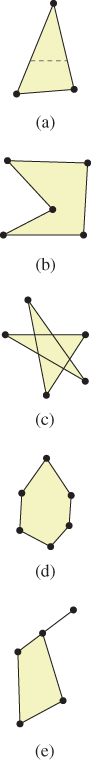
Figure 7.18: Polygons (a), (b), and (d) are simple, while (c) and (e) are not. Polygon (e) has a reflex vertex, (i.e., one with vertex angle zero) at the upper right.
7.10.1. Inside/Outside Testing
A polygon in the plane, in classic geometry, was simply a shape like the ones in Figure 7.18; because we attach an order to the vertices, we have slightly more structure. This allows us to define inside and outside for a larger class of polygons. Suppose that (P0, P1, ..., Pn) is a polygon. The line segments P0P1, P1P2, etc., are the edges of the polygon; the vectors v0 = P1 – P0, v1 = P2 – P1, ... vn = P0 – Pn are the edge vectors of the polygon.5 For each edge PiPi+1, the inward edge normal is the vector ×vi; the outward edge normal is – × vi. For a convex polygon whose vertices are listed in counterclockwise order, the inward edge normals point toward the interior of the polygon, and the outward edge normals point toward the unbounded exterior of the polygon, corresponding to our ordinary intuition. But if the vertices of a polygon are given in clockwise order, the interior and exterior swap roles. This is convenient in many situations. For example, imagine a polygon-shaped hole in a piece of metal. The interior of this polygon can (by suitable ordering of the vertices) be made to be the rest of the metal sheet. A light ray, trying to get from one side of the metal sheet to the other, is occluded exactly if it meets the interior of this polygon.
5. It’s convenient to write vi = Pi+1 – Pi, i = 0, ..., n; unfortunately, this formula fails at i = n because Pn+1 is undefined. Henceforth, it will be understood that in cases like this, Pn+1 = P0, Pn+2 = P1, etc. In other words, we continue the labeling cyclically; the same goes for indices less than zero: P–1 = Pn.
We can test whether a point in the plane is in the interior or exterior of a polygon, as shown in Figure 7.19, by casting a ray from the point in any direction. We find all intersections of the ray with polygon edges, and classify each as either entering (if the direction vector of the ray and the outward edge normal for the edge have a positive inner product) or leaving (if the inner product is negative). A point with more leaving intersections than entering ones is inside. Indeed, the difference between the number of leaving intersections and the number of entering intersections is called the winding number of the polygon about the point, and captures the notion of “how many times the polygon wraps around the point, counting counterclockwise.” The simple description above depends on the intersections of the ray and the polygon being a finite set. It doesn’t work when the ray actually contains an entire edge, and the answer, when the test point lies on an edge, depends on one’s definition of the intersection of a ray and a segment (as does the answer when the ray passes through a vertex of the polygon). This ray-casting approach to computing the winding number implicitly uses a strong theorem that says that the ray-casting computation results in the same value as the computation of the winding number itself, which is defined in a very different way: For a polygon with vertices P1, P2, ..., Pn, the winding number about a point Q is defined by considering the angles between successive rays from Q to each Pi. If these angles sum to 2π, the winding number is 1; if they sum to 4π, it’s 2, etc. Formally,
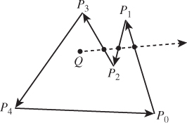
Figure 7.19: To test whether Q is in the interior of the polygon, we cast a ray in an arbitrary direction, and then count entering and leaving intersections with the edges. In this case, there are two leaving intersections (the first and third) and one entering intersection, so the point is inside.
Note that this is undefined if Q happens to be one of the vertices Pi, because the denominator is then zero. We also treat it as undefined when the argument to cos–1 is –1; this occurs when Q is on an edge of the polygon.
With these various definitions of the winding number, one can think of a curve as dividing the plane into a collection of regions. Within each region, the winding number is a constant; the labeling of regions by their winding numbers goes back to Listing, a student of Gauss [Lis48].
(a) Develop a small program to test whether a point is in the interior of a convex polygon by testing whether it’s strictly on the proper side of each edge. What’s the running time in terms of the number n of polygon vertices? (b) Assuming that you want to test many points to determine whether they’re inside or outside a single convex polygon, you can afford to do some preprocessing. Using a ray-casting test like the one described in this chapter, and a horizontal ray, show how you can create an O(log n) algorithm for inside/outside testing. Hint: Because the polygon is convex, you need only test ray intersection with a small number of edges. If you sort the vertices by their y-coordinates, how can you quickly find those edges?
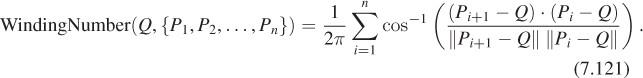
7.10.2. Interiors of Nonsimple Polygons
Most of the polygons we’ll encounter will be triangles, and therefore simple. But occasionally we’ll encounter nonsimple polygons in the plane, and there are several alternatives (see Figure 7.20) for defining the interior of these. All first compute the winding number of the polygon about the point P as before; in this case, though, the winding number may be different from one or zero. The positive winding number rule says that points with positive winding numbers are inside; the odd winding number rule says that those with odd winding numbers are inside—the result is a checkerboardlike appearance for the inside and outside regions; the nonzero winding number rule says that points with nonzero winding numbers are inside. Each has its uses; drawing programs should probably allow all three as alternatives.
Figure 7.20: (a) A nonsimple polygon whose regions have been labeled by Listing’s rule, (b) the interior defined by the positive winding number rule, (c) by the even-odd rule, and (d) by the nonzero winding number rule.
7.10.3. The Signed Area of a Plane Polygon: Divide and Conquer
If P1 = (x1, y1) and P2 = (x2, y2) are points in the xy-plane (see Figure 7.21), and Q = (0, 0) is the origin, then the signed area of the triangle QP1P2 is given by
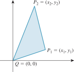
Figure 7.21: The signed area of the triangle QP1P2 is positive if the path from Q to P1 to P2 to Q is counterclockwise, and negative if it’s clockwise. In the example shown, the signed area is positive.
The signed area is positive if the vertices Q, P1, P2 are in counterclockwise order around the triangle, and negative if they’re in clockwise order. (It will be easy to prove this after you read Chapter 10, which discusses transformations in the plane: You first verify that the formula doesn’t change when the triangle is rotated, so you can assume that P1 lies on the positive x-axis, and therefore, P1 = (x1,0) with x1 > 0. The triangle is then clockwise if and only if P2 = (x2, y2) is in the y > 0 half-space, that is, y2 > 0. But the area formula then gives the area as ![]() x1y2 > 0. The clockwise case is similarly easy to verify.)
x1y2 > 0. The clockwise case is similarly easy to verify.)
From this formula for the area of a triangle, we can write a formula for the signed area of a triangle with vertices P0 = (x0, y0), P1 = (x1, y1), and P2 = (x2, y2): If we change to a coordinate system based at P0, the new coordinates of P1 and P2 are (x1 – x0, y1 – y0) and (x2 – y0, y2 – y0). Applying the formula to these coordinates gives
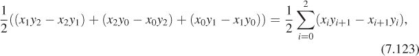
where indices are considered modulo 3, so x3 means x0 and y3 means y0.
To find the (signed) area of a polygon P0P1 ... Pn, we can use the same technique (see Figure 7.22): We compute the signed area of QP0P1, of QP1P2, ..., and of QPnP0; the parts of those areas that are outside the polygon cancel, while the ones inside add up to the correct total area. The final form is
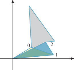
Figure 7.22: The pale yellow triangle is negatively oriented; the blue one positively. The next three will be negative, positive, and negative, and their signed areas will sum to give the gray polygon’s area.
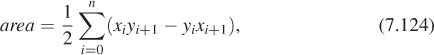
where xn+1 denotes x0 (i.e., the indices are taken modulo (n + 1)).
7.10.4. Normal to a Polygon in Space
A triangle P0P1P2 in space has a normal n as we computed earlier, given by n = (P1 – P0) × (P2 – P1). We could use this formula to compute the normal to a polygon in space as well, applying it to three successive vertices. But if these vertices happen to be collinear, we’ll get n = 0.
A more interesting approach, essentially due to Plücker [Plü68], is based on projected areas (see Figure 7.23 for an example where the polygon is a triangle): If one projects the polygon to the xy-, yz-, and zx-planes, one gets three planar polygons, each of whose areas can be computed; call these Axy, Ayz, and Azx. The normal vector to the polygon is then
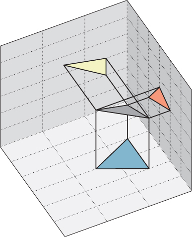
Figure 7.23: The gray triangle projects to three triangles, one in each coordinate plane. The signed areas of the orange, yellow, and blue triangles form the coordinates for the normal vector to the gray triangle.
this is not generally a unit vector. In fact, its length is the area of the polygon.
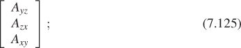
We can see this, in the case that the polygon is a triangle, by examining coordinates: If Pi = (xi, yi, zi) for i = 0, 1, 2, then n1, the first entry of the cross product, is just
The area formula for a plane polygon, Equation 7.124, applied to the projection of P0P1P2 to the yz-plane, gives

The eight terms in the expansion of the expression for n1 match the six terms in the expression for 2Axy because two y1z1 terms have opposite signs and cancel. The computations for n2 and n3 are similar. Thus, the vector
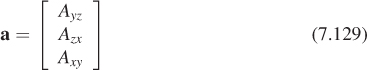
is twice the cross product; since half the length of the cross product is that triangle area, we see that the length of a is the triangle area.
The more general case follows by decomposing the polygon into a union of triangles.
The advantage of Plücker’s formula as applied to polygons in space is that if there are small numerical errors in the coordinates of a single vertex, they have relatively little impact on the computed normal vector.
7.10.5. Signed Areas for More General Polygons
If we have a polygon P0P1 ... Pn in a plane S whose normal is the unit vector n, we can find two orthogonal unit vectors x and y in S such that x, y, n is positively oriented, that is, n = x × y. Choosing some point of the plane as the origin, we have a coordinate system. We can then write the coordinates of each Pi in the xyn-coordinate system; the third coordinate will be zero, so the coordinates of Pi will be (xi, yi,0). We can apply the formula for a signed area to these coordinates. In the case of a triangle, if the signed area is positive (resp. negative), we say that the triangle is positively (resp. negatively) oriented. Notice, though, that if we had used – n instead of n, the signs would have changed: The signed area, and the orientation of a triangle, are only defined relative to a plane-with-normal.
Just as in the case of the xz-plane, a triangle is positively oriented in a plane with normal n if, as we look from the tip of n toward the plane, the vertices of the triangle appear in counterclockwise order.
When we speak of the signed area of a polygon in the zx-plane, we mean that we’re using a coordinate system in which the first basis vector is [0 0 1]T, the second is [1 0 0]T, and the normal vector is [0 1 0]T; a parallel description applies to the xy- and yz-planes.
Confirm that this definition of signed area for a triangle in an arbitrary plane in 3-space agrees with our definition of signed area for a triangle in the xy-plane.
7.10.6. The Tilting Principle
One situation that arises repeatedly in computer graphics is shown in Figure 7.24: We have a triangle T′ in a plane P′ with unit normal n′, and we project it to a triangle T in a plane P with unit normal n, the projection being along n. For instance, if P is the zx-plane, the projection is along the y-axis, taking (a, b, c) to (a,0, c).
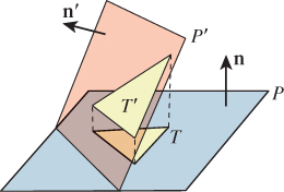
The (signed) areas of T′ and T are related by a cosine.
We call this the tilting principle.
![]() The Tilting Principle
The Tilting Principle
If T′ is an oriented triangle in plane P′ with normal n′, and T is its projection to plane P, the projection being along the unit normal n to P, then the signed area of T is n′ · n times the signed area of T′.
Once we’ve shown that the tilting principle applies to triangles, it also will apply to a polygon and its projection: We simply triangulate the polygon, and form a corresponding triangulation on its projection, and consider the area ratios one triangle at a time.
We’ll prove this claim about the ratio of signed areas for the case where the plane P is the xz-plane, and the triangle T′ has vertices A′, B′, and C′ with coordinates (ax, ay, az), etc.; the corresponding vertices of T are A = (ax, 0, az), etc.
Proving the principle in this special case is sufficient. We can always choose a coordinate system for space that makes the plane P be the xz-plane. Furthermore, we can rotate the coordinate system until the x-coordinate of the unit normal n′ to T′ is zero. Figure 7.25 shows this situation.
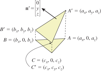
The vector n′ has the form [0 y z]T and length 1, so y2 + z2 = 1. Letting θ = atan2(y, z), we can write n′ = [0 cos θ sin θ]T. The dot product of n′ with the xz-plane’s unit normal n = [0 1 0]T is exactly cos θ.
Let’s compute the two signed areas. For T, the formula is
For T′, the (unsigned) area is the length of the vector a′ = [A′yz, A′zx, A′xy]. Because T′ is tilted only in the yz-plane, A′yz = 0. And because the x- and z-coordinates for T and T′ agree, we have
That leaves only A′xy to consider:
Remembering that the normal to the plane of T′ is [0 cos θ sin θ]T, we know the plane equation: Every point (x, y, z) on this plane must satisfy
where K is some constant. (You should make sure that you understand why this is true.) This means that for any point (x, y, z) on the plane,
Applying this to ay, by, and cy in Equation 7.132 and canceling many terms, we get
The length of a′ (hence the area of T′) is thus
while the area of T is |Azx|. Thus, the area of T′ is | cos θ| times that of T′.
There remains the question of the sign. If cos θ > 0, and the signed area of ΔA′ B′ C′ is positive, then the vertices A, B, and C are organized counterclockwise as viewed from the tip of n, and hence the signed area of Δ ABC is also positive. On the other hand, if cos θ < 0 and the signed area of Δ A′ B′ C′ is positive, then the vertices A, B, and C as viewed from the tip of n are organized clockwise, and hence the signed area of Δ ABC is negative. If we reverse the order of A, B, and C, in both cases, both signed areas change sign. So, in all four possible cases, the ratio of unsigned areas is | cos θ |, and the sign of the ratio of signed areas is the sign of cos θ, hence the ratio of signed areas is exactly cos θ = n · n′.
Suppose that instead of projecting T′ onto the xy-plane by projecting in the y-direction, we projected in the n′ direction. What would be the relationship between the signed area of the projected triangle T″ and that of T′?
7.10.7. Analogs of Barycentric Coordinates
![]() Barycentric coordinates provide a very useful way to discuss point locations within a triangle, because they are invariant under affine transformations. That is, if the point Q has barycentric coordinates (s0, s1, s2) in the triangle P0P1P2, and we transform the triangle by applying the same transformation T to each Pi and to Q, and if T is an affine transformation—that is, a rotation, a translation, a dilation, or a combination of these—then the barycentric coordinates of T(Q) in the triangle T(P0)T(P1)T(P2) will still be (s0, s1, s2). Furthermore, on the edge between P0 and P1, we have s2 = 0, and similarly for the other two edges. The barycentric coordinates are all positive for points inside the triangle, but for any point outside the triangle, at least one barycentric coordinate is negative. Is there an analogous set of “coordinates” for a point in a polygon? Warren and others have studied this question extensively, developing generalized barycentric coordinates for points in a convex polygon or set [War96] [WSHD04] and a generalization to coordinates that use all points of a mesh to define coordinates on points in and around that mesh [JSW05].
Barycentric coordinates provide a very useful way to discuss point locations within a triangle, because they are invariant under affine transformations. That is, if the point Q has barycentric coordinates (s0, s1, s2) in the triangle P0P1P2, and we transform the triangle by applying the same transformation T to each Pi and to Q, and if T is an affine transformation—that is, a rotation, a translation, a dilation, or a combination of these—then the barycentric coordinates of T(Q) in the triangle T(P0)T(P1)T(P2) will still be (s0, s1, s2). Furthermore, on the edge between P0 and P1, we have s2 = 0, and similarly for the other two edges. The barycentric coordinates are all positive for points inside the triangle, but for any point outside the triangle, at least one barycentric coordinate is negative. Is there an analogous set of “coordinates” for a point in a polygon? Warren and others have studied this question extensively, developing generalized barycentric coordinates for points in a convex polygon or set [War96] [WSHD04] and a generalization to coordinates that use all points of a mesh to define coordinates on points in and around that mesh [JSW05].
7.11. Discussion
The lessons to take away from this chapter are as follows.
• Be careful to say what you mean precisely when you use mathematics. Give your functions both domains and codomains; examine what happens when a formula could lead to a division by zero; and generalize to n dimensions whenever possible to better understand the intrinsic nature of the problem you’re solving.
• Whenever possible, express computations that need to be done in R2 or R3 as vector computations, involving vector operations, point-vector combinations, point-point differences, and inner products, and thereby avoid per-coordinate expressions.
• Try to understand geometric problems geometrically rather than in terms of coordinates; use coordinates for computations only.
These approaches lead to clearer understanding and more easily maintainable programs, and can often lead to insights about algorithms because the compactness of well-expressed mathematics allows us to see patterns that might otherwise be obscure.
7.12. Exercises
Exercise 7.1: (a) Show that if s is a number and v is a vector, then ||sv|| = |s|||v||;. (b) Give an example of a number s and vector v for which ||sv|| ≠ s||v||.
Exercise 7.2: We showed how to get from a point P on a line and a vector n normal to the line to the more familiar Ax + By + C = 0 form. Figure out how to go the other way: Given a line defined by Ax + By + C = 0, with at least one of A and B nonzero, find a point on the line. Hint: A normal vector to the line is given by ![]() . Use this to determine a point of the form O + αn (where O is the origin) that lies on the line, by solving for α.
. Use this to determine a point of the form O + αn (where O is the origin) that lies on the line, by solving for α.
Exercise 7.3: The expression u · (×v) that arose in studying line intersections occurs quite often (as do its generalizations to higher dimensions). Show that it equals the determinant of a matrix whose first column is v and whose second column is u. As a point of information, this works more generally: In 3-space, u · (v × w) is the same as the determinant of a matrix whose columns are v, w, and u and similar formulas hold in higher dimensions.
Exercise 7.4: Find the parametric form of the line between the points (1, 1) and (2, 2). Then find the parametric form of the line between the points (3, 3) and (5, 5). Are the two functions identical? Are the lines they describe identical? Explain why the mapping defined by the parametric line formula is actually a map from “two distinct points in the plane” to “a parametric representation of the line between these points,” rather than from the line itself to a parametric representation.
Exercise 7.5: The same reasoning as in Exercise 7.4 applies to the implicit form of a line: Depending on the points chosen, we get different “standard implicit forms.” Fortunately, all define the same line. Furthermore, any two standard implicit forms are proportional. Write down the implicit form of the line between the points (1, 1) and (2, 2). Then find the implicit form of the line between the points (3, 3) and (5, 5). Are the two implicit functions identical? Are they proportional? Are the points where they are zero identical?
Exercise 7.6: Since any two standard implicit forms of a line are proportional, is there a way to choose a “standard representative” once and for all? Suppose that Ax + By + C and A′ x + B′ y + C′ = 0 describe the same line. Then we know that the triples (A, B, C) and (A′, B′, C′) are proportional, and that any other triple proportional to these (except (0,0,0)) will determine the same line. Can we choose just one and call it the “normal form of the line”? For instance, we might say, “Take your triple (A, B, C) and convert to a normal form where B = 1 by dividing through by B to get (A/B, 1, C/B).” Unfortunately, this doesn’t work if B = 0; the same goes for A and C. We can take the triple (A, B, C) and divide by ![]() to get a “normal form”; if we do this, the only ambiguity is a sign: The standard form for (A, B, C) and the one for (–A, –B, –C), which determine the same line, end up being opposites. Explain why (a) if λ ≠ 0, the lines determined by (A, B, C) and (λA, λB, λC) are identical; (b) if λ > 0, they have the same normal form; and (c) the factor
to get a “normal form”; if we do this, the only ambiguity is a sign: The standard form for (A, B, C) and the one for (–A, –B, –C), which determine the same line, end up being opposites. Explain why (a) if λ ≠ 0, the lines determined by (A, B, C) and (λA, λB, λC) are identical; (b) if λ > 0, they have the same normal form; and (c) the factor ![]() is never zero when Ax + By + C = 0 determines a line.
is never zero when Ax + By + C = 0 determines a line.
Exercise 7.7: Barycentric coordinates can be used to describe lines within a triangle PQR. For instance, all points on the line PQ satisfy the equation γ = 0 (where α, β, and γ are the barycentric coordinates). Let S be a point that’s one-third of the way from P to Q, and consider the line passing through S and R. What equation, in barycentric coordinates, determines this line? (Hint: Draw a picture, and find the barycentric coordinates of at least two points on the line.)
Exercise 7.8: The inequality 4x + 2y – 6 ≥ 0 defines a half-plane; its boundary is the line ![]() consisting of solutions to 4x + 2y – 6 = 0. Find the point of
consisting of solutions to 4x + 2y – 6 = 0. Find the point of ![]() that’s on the x-axis, and the point of
that’s on the x-axis, and the point of ![]() that’s on the y-axis. Is the origin in the half-space defined by the inequality? Draw the normal ray for the equation of
that’s on the y-axis. Is the origin in the half-space defined by the inequality? Draw the normal ray for the equation of ![]() , and verify that it points toward the positive half-space, as described in Section 7.9.3.
, and verify that it points toward the positive half-space, as described in Section 7.9.3.
Exercise 7.9: Generalize to 3-space the result about normal vectors and the defining equation for half-planes: that for the half-plane defined by Ax + By + C ≥ 0, the vector ![]() points from the edge of the half-plane into the positive half-plane.
points from the edge of the half-plane into the positive half-plane.
![]() Exercise 7.10: The winding number of a parametric curve γ about a point z0 of the complex plane is defined as
Exercise 7.10: The winding number of a parametric curve γ about a point z0 of the complex plane is defined as
Show that by parameterizing each edge of the polygon with vertices P1, ..., Pn with an interval of length 1, and treating the point with coordinates (x, y) as the complex number x + iy, we can reduce this integral definition to the simplified one we gave for polygons.
Exercise 7.11: (a) Show that the normal vector to a triangle with vertices P0, P1, P2 computed by Plücker’s method is indeed perpendicular to P1 – P0; a similar computation works to show it’s perpendicular to P2 – P0.
(b) Verify that for P0 = (0, 0, 0), P1 = (1, 0, 0), and P2 = (0, 1, 0), the normal computed by Plücker’s method points along the positive z-axis so that the vectors P2 – P0, P1 – P0, and n form a right-handed coordinate system.
![]() (c) Explain why the conclusion of part (b) holds regardless of the location of P0, P1, and P2, as long as they do not lie on a single line.
(c) Explain why the conclusion of part (b) holds regardless of the location of P0, P1, and P2, as long as they do not lie on a single line.
Exercise 7.12: Let P0P1P2 be a triangle in 3-space, and n its Plücker normal. Thinking of n as a covector, consider the function v ![]() n · v. What is its value on vectors lying in the plane of the triangle?
n · v. What is its value on vectors lying in the plane of the triangle?
Exercise 7.13: The inside-outside test for polygons based on ray intersections depends on the ray intersecting each edge in a single point. It also depends on the ray not passing through any polygon vertex, because if it did so, the intersections with both of the edges at the vertex would be counted. How can we avoid these problems?
(a) A randomized algorithm, in which the ray direction is chosen randomly, will fail with probability zero (assuming we are using infinite-precision numbers). If the chosen ray is a failure case, we can randomly choose a new one, and with probability one the algorithm will finish.
(b) We can find the set of all direction vectors of all edges in the polygon, and of all rays from the test point to all polygon vertices, and choose a direction which is different from all of these. Explain why, in the case of a very small quadrilateral, with vertices at (±ε, 0) and (0, ±ε), where ε is the smallest floating-point number representable on the computer, and with a test point Q at the origin, both of these approaches fail in practice. Will the more complex sum-of-inverse-cosines formula for computing the winding number work in this case?
Exercise 7.14: (To do this exercise, you’ll need to know something about transformations of the plane; these will be covered in Chapter 10.)
(a) Show that the area formula in Equation 7.122 is correct when P1, P2, and Q do not lie on a line, and when P1 is not on the y-axis, by doing two transformations: Shear in y to move P1 to the x-axis; then shear in x to move P2 to the y-axis. Show that shearing doesn’t change the computed area; Cavalieri’s principle shows that it doesn’t change the actual area.
(b) Show that the formula is right for the two remaining cases by presenting an argument for each. The formula for area is a continuous function of the coordinates of P1, P2, and Q. The actual area is also a continuous function of these coordinates. At this point we have shown that these two functions agree almost everywhere (e.g., whenever the three points do not lie on a line). By a continuity argument, they must therefore agree everywhere.
![]() (c) Show that the formula is correct by arguing that area is a continuous function of coordinates, and that there is, at most, one extension of a continuous function on X to a continuous function on X
(c) Show that the formula is correct by arguing that area is a continuous function of coordinates, and that there is, at most, one extension of a continuous function on X to a continuous function on X ![]() boundary(X) when X is a subset of Rn.
boundary(X) when X is a subset of Rn.
Exercise 7.15: Another approach to generalizing the area formula from the “one vertex at the origin” case to the general case is this: Compute the signed area of the triangle P0P1P2 by computing the signed areas of QP0P1, QP1P2, and QP2P0 and then adding or subtracting appropriately. Draw a picture to figure out what the relationship among the four signed areas should be, and use it to derive the general formula for the signed area of P0P1P2.
Exercise 7.16: Numerical considerations: In the formula for the area of a polygon, suppose that we are using finite precision arithmetic and we add L, where L is a very large number, to the x-coordinates of all the polygon’s vertices. What happens to the computation? What if we instead perform the computation by writing the coordinates of the vertices in a coordinate system based at the “center” of the polygon—the average of all the vertices?
Exercise 7.17: Consider a ray that starts at P = (–3, –3) and has direction ![]() . It intersects the ellipse defined by
. It intersects the ellipse defined by ![]() at two points. To find these points, we can write
at two points. To find these points, we can write
where the T indicates transpose. If we solve the second equation for t, we will have found the parameters t1 and t2 of the intersection points, from which we can compute the points.
(a) Draw a picture representing this situation.
(b) Confirm that the equations above really do determine the points of intersection by writing out the product explicitly.
(c) Now consider the intersection of the ray defined by the point Q = (–1, –3) and the direction ![]() , with the unit circle. Once again, draw a picture and express this problem as a similar pair of equations; the matrix in this case will be the identity matrix.
, with the unit circle. Once again, draw a picture and express this problem as a similar pair of equations; the matrix in this case will be the identity matrix.
(d) Expand these latter equations; compare them to the ones you arrived at in part (b).
(e) Explain the similarity: How are d and e related? How are the ellipse and the unit circle related? We’ll return to this kind of transformation from a general problem (compute an intersection with an ellipse) to an equivalent standard problem (compute an intersection of a different ray with the unit circle) when we study ray tracing.
Exercise 7.18: The function γ : R ![]() R2 : t
R2 : t ![]() (3 + 2t, 4 – 3t) describes a line in parametric form.
(3 + 2t, 4 – 3t) describes a line in parametric form.
(a) Find two distinct points P and Q on the line. (There are an infinite number of correct answers to this part.)
(b) Use these two to find an implicit form for the line; convert via algebra to the form Ax + By + C = 0.
Exercise 7.19: (a) You’re given two nondegenerate line segments in the plane, the first with endpoints A and B and the second with endpoints C and D, and all coordinates are integers. Your job is to determine whether the segments intersect, and the intersection point, if any.
(a) Write a short program to do this. If the segments are parallel, there are three cases: They’re disjoint (return false), they share an endpoint (return false), or they overlap in an interval (return true, but don’t return an intersection point, since it’s not unique). If the segments are nonparallel and intersect, they may share an endpoint (return false), the endpoint of one may be interior to the other (return true, and the endpoint), or the interiors of the segments may intersect at some point (x, y) whose coordinates may not be integers, but will be rational numbers. In this case, you should return an integer triple (x, y, w), where the intersection is at (x/w, y/w).
(b) Explain why returning an integer triple is more useful than returning a floating-point representation of the rational coordinates.
(c) Suppose you have two integer triples of the form above, (x1, y1, w1) and (x2, y2, w2). How would you test them for “equality,” that is, how would you test whether they represent the same rational point in the plane?
(d) For an extra challenge, try to write all your code in part (a) so that there are no divisions, and the code is as clean as possible. The sort of multiple-case mess that’s implicit in programs like this arises from the multiple possible ways that segments can intersect; you can’t really make the code too clean.