
CHAPTER 21 Image Transformations and Camera Calibration
21.1 Introduction
When images are obtained from 3-D scenes, the exact position and orientation of the camera sensing device are often unknown, and there is a need for it to be related to some global frame of reference. This is especially important if accurate measurements of objects are to be made from their images, for example, in inspection applications. On the other hand, it may sometimes be possible to dispense with such detailed information—as in the case of a security system for detecting intruders, or a system for counting cars on a motorway. There are also more complicated cases, such as those in which cameras can be rotated or moved on a robot arm, or the objects being examined can move freely in space. In such cases, camera calibration becomes a central issue. Before we can consider camera calibration, we need to understand in some detail the transformations that can occur between the original world points and the formation of the final image. We attend to these image transformations in the following section, and we then move on to details of camera parameters and camera calibration in the subsequent two sections. Then, in Section 21.5 we consider how any radial distortions of the image introduced by the camera lens can be corrected.
Section 21.6 signals an apparent break with the previous work and introduces ‘multiple view’ vision. This topic has become important in recent years, for it uses new theory to bypass the need for formal camera calibration, making it possible to update the vision system parameters during actual use. The basis for this work is generalized epipolar geometry. This takes the epipolar line ideas of Section 16.3.2 considerably further. At the core of this new work are the ‘essential’ and ‘fundamental’ matrix formulations, which relate the observed positions of any point in two camera frames of reference. Short sections on image ‘rectification’ (obtaining a new image as it would be seen from an idealized camera position) and 3-D reconstruction follow.
21.2 Image Transformations
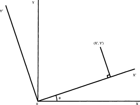
First, we consider the rotations and translations of object points relative to a global frame. After a rotation through an angle θ about the Z-axis (Fig. 21.1), the coordinates of a general point (X, Y) change to:
This result is neatly expressed by the matrix equation:
Similar rotations are possible about the X- and Y-axes. To satisfactorily express rotations in 3-D, we require a more general notation using 3 × 3 matrices, the matrix for a rotation θ about the Z-axis being:
 (21.4)
those for rotations ψ about the X-axis and φ about the Y-axis are:
 (21.5)
 (21.6)
We can make up arbitrary rotations in 3-D by applying sequences of such rotations. Similarly, we can express arbitrary rotations as sequences of rotations about the coordinate axes. Thus R = X(ψ)Y(φ)Z(θ) is a composite rotation in which Z(θ) is applied first, then Y(φ), and finally X(ψ). Rather than multiplying out these matrices, we write down here the general result expressing an arbitrary rotation R:
 (21.7)
Note that the rotation matrix R is not completely general. It is orthogonal and thus has the property that R-1 = RT.
In contrast with rotation, translation through a distance (T1, T2, T3) is given by:
which is not expressible in terms of a multiplicative 3 × 3 matrix. However, just as general rotations can be expressed as rotations about various coordinate axes, so general translations and rotations can be expressed as sequences of basic rotations and translations relative to individual coordinate axes. Thus, it would be most useful to have a notation that unified the mathematical treatment so that a generalized displacement could be expressed as a product of matrices. This is indeed possible if so-called homogeneous coordinates are used. To achieve this, the matrices must be augmented to 4 × 4. A general rotation can then be expressed in the form:
 (21.11)
while the general translation matrix becomes:
 (21.12)
The generalized displacement (i.e., translation plus rotation) transformation clearly takes the form:
 (21.13)
We now have a convenient notation for expressing generalized transformations, including operations other than the translations and rotations that account for the normal motions of rigid bodies. First we take a scaling in size of an object, the simplest case being given by the matrix:
introduces a shear in which an object line λ will be transformed into a line that is not in general parallel to λ. Skewing is another interesting transformation, being given by linear translations varying from the simple case:
Rotations can be regarded as combinations of scaling and skewing and are sometimes implemented as such (Weiman, 1976).
The other simple but interesting case is that of reflection, which is typified by:
This generalizes to other cases of improper rotation where the determinant of the top left 3 × 3 matrix is—1.
In all the cases discussed above, it will be observed that the bottom row of the generalized displacement matrix is redundant. In fact, we can put this row to good use in certain other types of transformations. Of particular interest in this context is the case of perspective projection. Following Section 15.3, equation (15.1), the equations for projection of object points into image points are:
Next we make full use of the bottom row of the transformation matrix by defining the homogeneous coordinates as (Xh, Yh, Zh, h) = (hX, hY, hZ, h), where h is a nonzero constant that we can take to be unity. To proceed, we examine the homogeneous transformation:
 (21.17)
Dividing by the fourth coordinate gives the required values of the transformed Cartesian coordinates (fX/Z, fY/Z, f).
Let us now review this result. First, we have found a 4 × 4 matrix transformation that operates on 4-D homogeneous coordinates. These do not correspond directly to real coordinates, but real 3-D coordinates can be calculated from them by dividing the first three by the fourth homogeneous coordinate. Thus, there is an arbitrariness in the homogeneous coordinates in that they can all be multiplied by the same constant factor without producing any change in the final interpretation. Similarly, when deriving homogeneous coordinates from real 3-D coordinates, we can employ any convenient constant multiplicative factor h, though we will normally take h to be unity.
The advantage to be gained from use of homogeneous coordinates is the convenience of having a single multiplicative matrix for any transformation, in spite of the fact that perspective transformations are intrinsically nonlinear. Thus, a quite complex nonlinear transformation can be reduced to a more straightforward linear transformation. This eases computer calculation of object coordinate transformations, and other computations such as those for camera calibration (see Section 21.3). We may also note that almost every transformation can be inverted by inverting the corresponding homogeneous transformation matrix. An exception is the perspective transformation, for which the fixed value of z leads merely to Z being unknown, and X, Y only being known relative to the value of Z (hence the need for binocular vision or other means of discerning depth in a scene).
21.3 Camera Calibration
We have shown how homogeneous coordinate systems are used to help provide a convenient linear 4 × 4 matrix representation for 3-D transformations (including rigid body translations and rotations) and nonrigid operations (including scaling, skewing, and perspective projection). In this last case, it was implicitly assumed that the camera and world coordinate systems are identical, since the image coordinates were expressed in the same frame of reference. However, in general the objects viewed by the camera will have positions that may be known in world coordinates, but that will not a priori be known in camera coordinates, since the camera will in general be mounted in a somewhat arbitrary position and will point in a somewhat arbitrary direction. Indeed, it may well be on adjustable gimbals, and may also be motor driven, with no precise calibration system. If the camera is on a robot arm, there are likely to be position sensors that could inform the control system of the camera position and orientation in world coordinates, though the amount of slack may well make the information too imprecise for practical purposes (e.g., to guide the robot toward objects).
These factors mean that the camera system will have to be calibrated very carefully before the images can be used for practical applications such as robot pick-and-place. A useful approach is to assume a general transformation between the world coordinates and the image seen by the camera under perspective projection, and to locate in the image various calibration points that have been placed in known positions in the scene. If enough such points are available, it should be possible to compute the transformation parameters, and then all image points can be interpreted accurately until recalibration becomes necessary.
The general transformation G takes the form:
 (21.18)
where the final Cartesian coordinates appearing in the image are (x, y, z) = (x, y, f). These are calculated from the first three homogeneous coordinates by dividing by the fourth:
However, as we know z, there is no point in determining parameters G31, G32, G33, G34. Accordingly we proceed to develop the means for finding the other parameters. Because only the ratios of the homogeneous coordinates are meaningful, only the ratios of the Gij values need be computed, and it is usual to take G44 as unity: this leaves only eleven parameters to be determined. Multiplying out the first two equations and rearranging give:
Noting that a single world point (X, Y, Z) that is known to correspond to image point (x, y) gives us two equations of the above form; it requires a minimum of six such points to provide values for all 11 Gij parameters. Figure 21.2 shows a convenient near-minimum case. An important factor is that the world points used for the calculation should lead to independent equations. Thus it is important that they should not be coplanar. More precisely, there must be at least six points, no four of which are coplanar. However, further points are useful in that they lead to overdetermination of the parameters and increase the accuracy with which the latter can be computed. There is no reason why the additional points should not be coplanar with existing points. Indeed, a common arrangement is to set up a cube so that three of its faces are visible, each face having a pattern of squares with 30 to 40 easily discerned corner features (as for a Rubik cube).
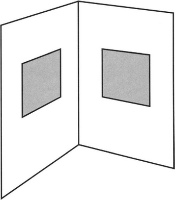
Figure 21.2 A convenient near-minimum case for camera calibration. Here two sets of four coplanar points, each set of four being at the corners of a square, provide more than the absolute minimum number of points required for camera calibration.
Least squares analysis can be used to perform the computation of the 11 parameters (e.g., via the pseudo-inverse method). First, the 2n equations have to be expressed in matrix form:
where A is a 2n x 11 matrix of coefficients, which multiplies the G-matrix, now in the form:
and ξ is a 2n-element column vector of image coordinates. The pseudo-inverse solution is:
The solution is more complex than might have been expected, since a normal matrix inverse is only defined, and can only be computed, for a square matrix. Note that solutions are only obtainable by this method if the matrix ATA is invertible. For further details of this method, see Golub and van Loan (1983).
21.4 Intrinsic and Extrinsic Parameters
At this point it is useful to look in more detail at the general transformation leading to camera calibration. When we are calibrating the camera, we are actually trying to bring the camera and world coordinate systems into coincidence. The first step is to move the origin of the world coordinates to the origin of the camera coordinate system. The second step is to rotate the world coordinate system until its axes are coincident with those of the camera coordinate system. The third step is to move the image plane laterally until there is complete agreement between the two coordinate systems. (This step is required since it is not known initially which point in the world coordinate system corresponds to the principal point 1 in the image.)
There is an important point to be borne in mind during this process. If the camera coordinates are given by C, then the translation T required in the first step will be—C. Similarly, the rotations that are required will be the inverses of those that correspond to the actual camera orientations. The reason for these reversals is that (for example) rotating an object (here the camera) forward gives the same effect as rotating the axes backwards. Thus, all operations have to be carried out with the reverse arguments to those indicated above in Section 21.1. The complete transformation for camera calibration is hence:
 (21.28)
where matrix P takes account of the perspective transformation required to form the image. It is usual to group together the transformations P and L and call them internal camera transformations, which include the intrinsic camera parameters, while R and T are taken together as external camera transformations corresponding to extrinsic camera parameters:
 (21.30)
 (21.31)
In the matrix for Ginternal we have assumed that the initial translation matrix T moves the camera’s center of projection to the correct position, so that the value of t3 can be made equal to zero: in that case, the effect of L will indeed be lateral as indicated above. At that point, we can express the 2-D result in terms of a 3 × 3 homogeneous coordinate matrix. In the matrix for Gexternal, we have expressed the result succinctly in terms of the rows R1, R2, R3 of R, and have taken dot-products with T(T 1; T2, T3,). The 3-D result is a 4 × 4 homogenous coordinate matrix.
Although the above treatment gives a good indication of the underlying meaning of G, it is not general because we have not so far included scaling and skew parameters in the internal matrix. In fact, the generalized form of Ginternal is:
 (21.32)
Potentially, Ginternal should include the following:
1. A transform for correcting scaling errors.
2. A transform for correcting translation errors.2
3. A transform for correcting sensor skewing errors (due to nonorthogonality of the sensor axes).
4. A transform for correcting sensor shearing errors (due to unequal scaling along the sensor axes).
5. A transform for correcting for unknown sensor orientation within the image plane.
Translation errors (item 2) are corrected by adjusting t1 and t2. All the other adjustments are concerned with the values of the 2 × 2 submatrix:
However, it should be noted that application of this matrix performs rotation within the image plane immediately after rotation has been performed in the world coordinates by Gexternal, and it is virtually impossible to separate the two rotations. This explains why we now have a total of six external and six internal parameters totaling 12 rather than the expected 11 parameters (we return to the factor 1/f below). As a result, it is better to exclude item 5 in the above list of internal transforms and to subsume it into the external parameters.3 Since the rotational component in Ginternal has been excluded, b1 and b2 must now be equal, and the internal parameters will be: s1, s2, b, t1, t2. Note that the factor 1/f provides a scaling that cannot be separated from the other scaling factors during camera calibration without specific (i.e., separate) measurement off. Thus, we have a total of six parameters from Gexternal and five parameters from Ginternal: this totals 11 and equals the number cited in the previous section.
At this point, we should consider the special case where the sensor is known to be Euclidean to a high degree of accuracy. This will mean that b = b1 = b2 = 0, and s1 = s2, bringing the number of internal parameters down to three. In addition, if care has been taken over sensor alignment, and there are no other offsets to be allowed for, it may be known that t1 = t2 = 0. This will bring the total number of internal parameters down to just one, namely, s = s1 = s2, or s/f, if we take proper account of the focal length. In this case there will be a total of seven calibration parameters for the whole camera system. This may permit it to be set up unambiguously by viewing a known object having four clearly marked features instead of the six that would normally be required (see Section 21.2).
21.5 Correcting for Radial Distortions
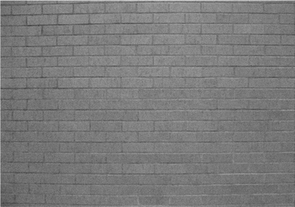
Photographs generally appear so distortion free that we tend to imagine that camera lenses are virtually perfect. However, it sometimes happens that a photograph will show odd curvatures of straight lines, particularly those appearing around the periphery of the picture. The results commonly take the form of ‘pincushion’ or ‘barrel’ distortion. These terms arise because pincushions have a tendency to be overextended at the corners, whereas barrels usually bulge in the middle. In images of paving stones or brick walls, the amount of distortion is usually not more than a few pixels in a total of the order of 512, that is, typically less than 2%. This explains why, in the absence of particular straight line markers, such distortions can be missed (Fig. 21.3). However, it is important both for recognition and for interimage matching purposes that any distortions be eliminated. Today image interpretation is targeted at, and frequently achieves, subpixel accuracy. In addition, disparities between stereo images are in the first order of small quantities, and single pixel errors would lead to significant errors in depth measurement. Hence, it is more the rule than the exception that 3-D image analysis will need to make corrections for barrel or pincushion distortion.
For reasons of symmetry, the distortions that arise in images tend to involve radial expansions or contractions relative to the optical axis—corresponding, respectively, to pincushion or barrel distortion. As with many types of errors, series solutions can be useful. Thus, it is worthwhile to model the distortions as:
the odd orders in the brackets canceling to zero, again for reasons of symmetry. It is usual to set a0 to unity, as this coefficient can be taken up by the scale parameters in the camera calibration matrix.
To fully define the effect, we write the x and y distortions as:
Here x and y are measured relative to the position of the optical axis of the lens (x<sub>c</sub>, y<sub>c</sub>), so r = (x—x<sub>c</sub>, y—y<sub>c</sub>), r’ = (x’—x<sub>c</sub>, y’—y<sub>c</sub>)-
As stated earlier, the errors to be expected are in the 2% or less range. That is, it is normally sufficiently accurate to take just the first correction term in the expansion and disregard the rest. At the very least, this will introduce such a large improvement in the accuracy that it will be difficult to detect any discepancies, especially if the image dimensions are 512 × 512 pixels or less.4 In addition, computation errors in matrix inversion and convergence of 3-D algorithms will add to the digitization errors, tending further to hide higher powers of radial distortion. Thus, in most cases the distortion can be modeled using a single parameter equation:
Note that the above theory only models the distortion; it has to be corrected by the corresponding inverse transformation.
It is instructive to consider the apparent shape of a straight line that appears, for example, along the top of an image (Fig. 21.3). Take the image dimensions to range over—x1 ![]() x
x ![]() x1,—y1
x1,—y1 ![]() y
y ![]() y1, and the optical axis of the camera to be at the center of the image. Then the straight line will have the approximate equation:
y1, and the optical axis of the camera to be at the center of the image. Then the straight line will have the approximate equation:
Clearly, it is a parabola. The vertical error at the center of the parabola is a2y13, and the additional vertical error at the ends is a2y1x.12 If the image is square (x1 = y1), these two errors are equal. (The erroneous impression is given by the parabola shape that the error at x = 0 is zero.)
Finally, note that digital scanners are very different from single-lens cameras, in that their lenses travel along the object space during acquisition. Thus, longitudinal errors are unlikely to arise to anything like the same extent, though lateral errors could in principle be problematic.
21.6 Multiple-view Vision
In the 1990s, a considerable advance in 3-D vision was made by examining what could be learned from uncalibrated cameras using multiple views. At first glance, considering the efforts made in earlier sections of this chapter to understand exactly how cameras should be calibrated, this may seem nonsensical. Nevertheless, there are considerable potential advantages in examining multiple views—not least, many thousands of videotapes are available from uncalibrated cameras, including those used for surveillance and those produced in the film industry. In such cases, as much must be made of the available material as possible, whether or not any regrets over ‘what might have been’ are entertained. However, the need is deeper than this. In many situations the camera parameters might vary because of thermal variations, or because the zoom or focus setting has been adjusted. It is impracticable to keep recalibrating a camera using accurately made test objects. Finally, if multiple (e.g., stereo) cameras are used, each will have to be calibrated separately, and the results compared to minimize the combined error. It is far better to examine the system as a whole, and to calibrate it on the real scenes that are being viewed.
We have already encountered some aspects of these aspirations, in the form of invariants that are obtained in sequence by a single camera. For example, if a series of four collinear points are viewed and their cross ratio is checked, it will be found to be constant as the camera moves forward, changes orientation, or views the points increasingly obliquely—as long as they all remain within the field of view. For this purpose, all that is required to perform the recognition and maintain awareness of the object (the four points) is an uncalibrated but distortion-free camera. By distortion-free here we mean not the ability to correct perspective distortion—which is, after all, the function of the cross ratio invariant—but the lack of radial distortion, or at least the capability in the following software for eliminating it (see Section 21.5).
To understand how image interpretation can be carried out more generally, using multiple views—whether from the same camera moved to a variety of places, or multiple cameras with overlapping views of the world—we shall need to go back to basics and start afresh with a more general attack on concepts such as binocular vision and epipolar constraints. In particular, two important matrices will be called into play—the ‘essential’ matrix and the ‘fundamental’ matrix. We start with the essential matrix and then generalize the idea to the fundamental matrix. But first we need to look at the geometry of two cameras with general views of the world.
21.7 Generalized Epipolar Geometry
In Section 16.3, we considered the stereo correspondence problem and had already simplified the task by choosing two cameras whose image planes were not only parallel but in the same plane. This made the geometry of depth perception especially simple but suppressed possibilities allowed for in the human visual system (HVS) of having a nonzero vergence angle between the two images. The HVS is special in adjusting vergence so that the current focus of attention in the field of view has almost zero disparity between the two images. It seems likely that the HVS estimates depth not merely by measuring disparity but by measuring the vergence together with remanent small variations in disparity.
Here we generalize the situation to cover the possibility of disparity coupled with substantial vergence. Figure 21.4 shows the revised geometry.
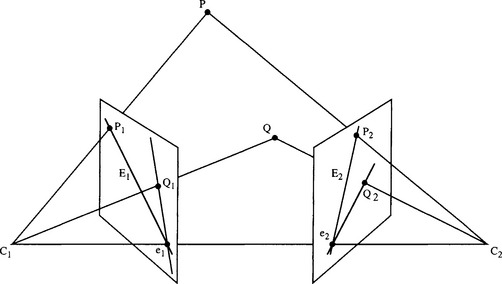
Figure 21.4 Generalized imaging of a scene from two viewpoints. In this case, there is substantial vergence. All epipolar lines in the left image pass through epipole e1; of these, only E1 is shown. Similar comments apply for the right image.
Note first that observation of a real point P in the scene leads to points P1 and P2 in the two images; that P1 could correspond to any point on the epipolar line E2 in image 2; and similarly, that point P2 could correspond to any point on the epipolar line E1 in image 1. The so-called epipolar plane of P is the plane containing P and the projection points C1 and C2 of the two cameras. The epipolar lines (see Section 16.3) are thus the straight lines in which this plane cuts the two image planes. Furthermore, the line joining C1 and C2 cuts the image planes in the so-called epipoles e1 and e2. These can be regarded as the images of the alternate camera projection points. Note that all epipolar planes pass through points C1, C2 and e1, e2. This means that all epipolar lines in the two images pass through the respective epipoles. However, if the vergence angle were zero (as in Fig. 16.5), the epipoles would be at infinity in either direction and all epipolar lines in either image would be parallel, and indeed parallel to the vector C from C1 to C2.
21.8 The Essential Matrix
In this section we start with the vectors P1, P2, from C1, C2 to P, and also the vector C from C1 to C2. Vector subtraction gives:
We also know that P1, P2 and C are coplanar, the condition of coplanarity being:5
To progress, we need to relate the vectors P1 and P2 when these are expressed relative to their own frames of reference. If we take these vectors as having been defined in the C1 frame of reference, we now reexpress P2 in its own (C2) frame of reference, by applying a translation C and a rotation of coordinates expressed as the orthogonal matrix R. This leads to:
Substituting in the coplanarity condition gives:
At this point it is useful to replace the vector product notation by using a skew-symmetrical matrix Cx to denote C x, where:
 (21.43)
At the same time we observe the correct matrix formulation of all the vectors by transposing appropriately. We now find that:
Finally, we obtain the ‘essential matrix’ formulation:
where the essential matrix has been found to be:
Equation (21.46) is actually the desired result: it expresses the relation between the observed positions of the same point in the two camera frames of reference. Furthermore, it immediately leads to formulas for the epipolar lines. To see this, first note that in the C1 camera frame:
while in the C2 camera frame (and expressed in terms of that frame of reference):
Eliminating P1 and P’2, and dropping the prime (as within the respective image planes the numbers 1 and 2 are sufficient to specify the coordinates unambiguously), we find:
as Z1, Z2 and f1, f2 can be canceled from this matrix equation.
Now note that writing p<sub>2</sub><sup>T</sup>E = l<sub>1</sub> and l2 = Ep1 leads to the following relations:
This means that l2 = E p1 and l1 = ETp2 are the epipolar lines corresponding to p1 and p2, respectively.6
Finally, we can find the epipoles from the above formulation. In fact, the epipole lies on every epipolar line within the same image. Thus, e2 satisfies (can be substituted for p2 in) equation (21.52), and hence:
This means that eT2E= 0, i.e., ETe2 = 0. Similarly, Ee1 = 0.
21.9 The Fundamental Matrix
Notice that in the last part of the essential matrix calculation, we implicitly assumed that the cameras are correctly calibrated. Specifically, p1 and p2 are corrected (calibrated) image coordinates. However, there is a need to work with uncalibrated images, using the raw pixel measurements 7—for all the reasons given in Section 21.6. Applying the camera intrinsic matrices G1, G2 to the calibrated image coordinates (Section 21.4), we get the raw image coordinates:
Here we need to go in the reverse direction, so we use the inverse equations:
Substituting for p1 and p2 in equation (21.50), we find the desired equation linking the raw pixel coordinates:
F is defined as the ‘fundamental matrix.’ Because it contains all the information that would be needed to calibrate the cameras, it contains more free parameters than the essential matrix. However, in other respects the two matrices are intended to convey the same basic information, as is confirmed by the resemblance between the two formulations—see equations (21.50) and (21.58).
Finally, just as in the case of the essential matrix, the epipoles are given by Ff1 = 0 and FTf2 = 0, though this time in raw image coordinates f1 and f2.
21.10 Properties of the Essential and Fundamental Matrices
Next we consider the composition of the essential and fundamental matrices. In particular, note that Cx is a factor of E and also, indirectly, of F. They are homogeneous in Cx, so the scale of C will make no difference to the two matrix formulations (equations (21.46) and (21.58)), with only the direction of C being important. The scales of both E and F are immaterial, and as a result only the relative values of their coefficients are of importance. This means that there are at most only eight independent coefficients in E and F. In the case of F there are only seven, asCx is skew-symmetrical, and this ensures that it has rank 2 rather than rank 3—a property that is passed on to F. The same argument applies for E, but it turns out that the lower complexity of E (by virtue of its not containing the image calibration information) means that it has only five free parameters. In the latter case, it is easy to see what they are: they arise from the original three translation (C) and three rotation (R) parameters, less the one parameter corresponding to scale.
In this context, it should be noted that if C arises from a translation of a single camera, the same essential matrix will result whatever the scale of C. Only the direction of C actually matters, and the same epipolar lines will result from continued motion in the same direction. In this case we can interpret the epipoles as foci of expansion or contraction. This underlines the power of this formulation: specifically, it treats motion and displacement as a single entity.
Finally, we should try to understand why there are seven free parameters in the fundamental matrix. The solution is relatively simple. Each epipole requires two parameters to specify it. In addition, three parameters are needed to map any three epipolar lines from one image to the other. But why do just three epipolar lines have to be mapped? This is because the family of epipolar lines is a pencil whose orientations are related by cross ratios, so once three epipolar lines have been specified the mapping of any other can be deduced. (Knowing the properties of the cross ratio, it is seen that fewer than three epipolar lines would be insufficient and that more than three would yield no additional information.) This fact is sometimes stated in the following form: a homography (a projective transformation) between two 1-D projective spaces has three degrees of freedom.
21.11 Estimating the Fundamental Matrix
In the previous section we showed that the fundamental matrix has seven free parameters. This means that it ought to be possible to estimate it by identifying the same seven features in the two images.8 Although this is mathematically possible in principle, and a suitable nonlinear algorithm has been devised by Faugeras et al. (1992) to implement it, it has been shown that the computation can be numerically unstable. Essentially, noise acts as an additional variable boosting the effective number of degrees of freedom in the problem to eight. However, a linear algorithm called the eight-point algorithm has been devised to overcome the problem. Curiously, Longuet-Higgins (1981) proposed this algorithm many years earlier to estimate the essential matrix, but it came into its own when Hartley (1995) showed how to control the errors by first normalizing the values. In addition, by using more than eight points, increased accuracy can be attained, but then a suitable algorithm must be found that can cope with the now overdetermined parameters. Principal component analysis can be used for this purpose, an appropriate procedure being singular value decomposition (SVD).
Apart from noise, gross mismatches in forming trial point correspondences between images can be a source of practical problems. If so, the normal least-squares types of solution can profitably be replaced by the least median of squares robust estimation method (Appendix A).
21.12 Image Rectification
In Section 21.7 we took some pains to generalize the epipolar approach, and we subsequently arrived at general solutions, corresponding to arbitrary overlapping views of scenes. However, there are distinct advantages in special views obtained from cameras with parallel axes—as in the case of Fig. 16.5 where the vergence is zero. Specifically, it is easier to find correspondences between scenes that are closely related in this way. Unfortunately, such well-prepared pairs of images are not in keeping with the aims promoted in Section 21.6, of insisting upon closely aligned and calibrated cameras. The frames taken by a single moving camera certainly do not match well unless the camera’s motion is severely constrained by special means. The solution is straightforward: take images with uncalibrated cameras, estimate the fundamental matrix, and then apply suitable linear transformations to compute the images for any desired idealized camera positions. This technique is called image rectification and ensures, for example, that the epipolar lines are all parallel to the baseline C between the centers of projection. This then results in correspondences being found by searching along points with the same ordinate in the alternate image. For a point with coordinates (x1, y1) in the first image, search for a matching point (x2, y1) in the second image.
When rectifying an image, it will in general be rotated in 3-D,9 and the obvious way of doing so is to transfer each individual pixel to its new location in the rectified image. However, rotations are nonlinear processes and will in some cases have the effect of mapping several pixels into a single pixel. Furthermore, a number of pixels may well not have intensity values assigned to them. Although the first of these problems could be tackled by an intensity averaging process, and the second problem by applying a median or other type of filter to the transformed image, such techniques are insufficiently thoroughgoing to provide accurate, reliable solutions. The proper way of overcoming these intrinsic difficulties is to back-project the pixel locations from the transformed image space to the source image, use interpolation to compute the ideal pixel intensities, and then transfer these intensities to the transformed image space.
Bilinear interpolation is used most often in the transformation process. This works by performing interpolation in the x-direction and then in the y-direction. Thus, if the location to be interpolated is (x + a, y + b) where x and y are integer pixel locations, and 0 < a, b < 1, then the interpolated intensities in the x-direction are:
and the final result after interpolating in the y-direction is:
The symmetry of the result shows that it makes no difference which axis is chosen for the first pair of interpolations, and this fact limits the arbitrariness of the method. Note that the method does not assume a locally planar intensity variation in 2-D—as is clear because the value of the I(x + 1, y + 1) intensity is taken into account as well as the other three intensity values. Nevertheless, bilinear interpolation is not a totally ideal solution, for it takes no account of the sampling theorem. For this reason the bi-cubic interpolation method (which involves more computation) is sometimes used instead. In addition, all such methods introduce slight local blurring of the image as they involve averaging of local intensity values. Overall, transformation processes such as this one are bound to result in slight degradation of the image data.
21.13 3-D Reconstruction
Section 21.10 strongly emphasized that F is determined only up to an unknown scale factor (or equivalently that the actual scales of its coefficients as obtained are arbitrary), thus reflecting the deliberate avoidance of camera calibration in this work. In practice this means that if the results of computations of Fare to be related back to the real world, the scaling factor must be reinstated. In principle, scaling can be achieved by viewing a single yardstick. It is unnecessary to view an object such as a Rubik cube, for knowledge of F carries with it a lot of information on relative dimensions in the real world. This factor is important when reconstructing a real scene with a real depth map.
A number of methods are avaliable for image reconstruction, of which perhaps the most obvious is triangulation. This method starts by taking two camera positions containing normalized images, and projecting rays for a given point P back into the real world until they meet. Attempting to do this presents an immediate problem: the inaccuracies in the available parameters, coupled with the pixellation of the images, ensure that in most cases rays will not actually meet, for they are skew lines. The best that can be done with skew lines is to determine the position of closest approach. Once this position has been found, the bisector of the line of closest approach (which is perpendicular to each of the rays) is, in this model, the most accurate estimate of the position of P in space.
Unfortunately, this model is not guaranteed to give the most accurate prediction of the position of P. This is because perspective projection is a highly nonlinear process. In particular, slight misjudgment of the orientation of the point from either of the images can cause a substantial depth error, coupled with a significant lateral error. So much is indeed obvious from Fig. 21.5. This being so, we must ask where the error might still be linear, so that, at that position at least, error calculation can be based on Gaussian distributions.10 The errors can be taken to be approximately Gaussian in the images themselves. Thus, the point in space that has to be chosen as representing the most accurate interpretation of the data is that which results in the minimum error (in a least mean square sense) when reprojected onto the image planes. Typically, the error obtained using this approach is a factor of two smaller than that for the triangulation method described earlier (Hartley and Zisserman, 2000).
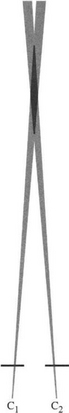
Figure 21.5 Error in locating a feature in space using binocular imaging. The dark shaded regions represent the regions of space that could arise for small errors in the image planes. The crossover region, shaded black, confirms that longitudinal errors will be much larger than lateral errors. A full analysis would involve applying Gaussian or other error functions (see text).
Finally, it is useful to mention another type of error that can arise with two cameras. This applies when they both view an object with a smoothly varying boundary. For example, if both cameras are viewing the right-hand edge of a vase of circular cross section, each will see a different point on the boundary and a discrepancy will arise in the estimated boundary position (Fig. 21.6). It is left as an exercise (Section 21.17) to determine the exact magnitude of such errors. The error is proportional both to a, where a is the local radius of curvature of the observed boundary, and to Z~2, where Z is the depth in the scene. This means that the error (and the percentage error) tends to zero at large distances, and that the error falls properly to zero for sharp corners.
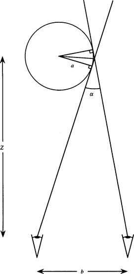
Figure 21.6 Lateral estimation error arising with a smoothly varying boundary. The error arises in estimating the boundary position when information from two views is fused in the standard way. a is the radius of a vase being observed, α is the disparity in direction of its right hand boundary, Z is its depth in the scene, and b is the stereo baseline.
21.14 An Update on the 8-point Algorithm
Section 21.11 outlined the value of the 8-point algorithm for estimating the fundamental matrix. Over a period of about eight years (1995-2003), this became the standard solution to the problem. However, a key contribution by Torr and Fitzgibbon (2003, 2004) has shown that the 8-point algorithm might not after all be the best possible method, since the solutions it obtains depend on the particular coordinate system used for the computation. This is because the normalization generally used, namely, ![]() 11 is not invariant to shifts in the coordinate system. It is by no means obvious how to find an invariant normalization. Nevertheless, Torr and Fitzgibbon’s logical analysis of the situation, in which they were forced to disregard the affine transform case appropriate for weak perspective, led to the following normalization of F:
11 is not invariant to shifts in the coordinate system. It is by no means obvious how to find an invariant normalization. Nevertheless, Torr and Fitzgibbon’s logical analysis of the situation, in which they were forced to disregard the affine transform case appropriate for weak perspective, led to the following normalization of F:
 (21.64)
Finally, to determine F, equation (21.63) can be applied as a Lagrangian multiplier constraint, which leads to an eigenvector solution for F. Overall, the 8 × 8 eigenvalue problem solved by the 8-point algorithm is replaced by a 5 × 5 eigenvalue problem. This approach not only yields the required invariance properties, thus ensuring a more accurate solution, but also gives a much faster computation that loses significantly fewer tracks in image sequence analysis.
21.15 Concluding Remarks
This chapter has discussed the transformations required for camera calibration and has outlined how calibration can be achieved. The camera parameters have been classified as internal and external, thereby simplifying the conceptual problem and throwing light on the origins of errors in the system. It has been shown that a minimum of 6 points are required to perform calibration in the general case where 11 transformation parameters are involved. However, the number of points required might be reduced somewhat in special cases, for example, where the sensor is known to be Euclidean. Nevertheless, it is normally more important to increase the number of points used for calibration than to attempt to reduce it, since substantial gains in accuracy can be obtained via the resulting averaging process.
In an apparent break with the previous work, Section 21.5 introduced multiple-view vision. This important topic was seen to rest on generalized epipolar geometry and led to the essential and fundamental matrix formulations, which relate the observed positions of any point in two camera frames of reference. The importance of the 8-point algorithm for estimating either of these matrices—and particularly the fundamental matrix, which is relevant when the cameras are uncalibrated—was stressed. In addition, the need for accuracy in estimating the fundamental matrix is still a research issue, with at least one new view of how it can be improved having been published as late as 2004 (Torr and Fitzgibbon, 2003, 2004).
The obvious way of tackling vision problems is to set up a camera and calibrate it, and only then to use it in anger. This chapter has shown how, to a large extent, calibration can be avoided or carried out adaptively ‘on the fly,’ by performing multiple-view vision and analyzing the various key matrices that arise from the generalized epipolar problems.
21.16 Bibliographical and Historical Notes
One of the first to use the various transformations described in this chapter was Roberts (1965). Important early references for camera calibration are the Manual of Photogrammetry (Slama, 1980), Tsai and Huang (1984), and Tsai (1986). Tsai’s paper is especially useful in that it provides an extended and highly effective treatment that copes with nonlinear lens distortions. More recent papers on this topic include Haralick (1989), Crowley et al. (1993), Cumani and Guiducci (1995), and Robert (1996): see also Zhang (1995). Note that parametrized plane curves can be used instead of points for the purpose of camera calibration (Haralick and Chu, 1984).
Camera calibration is an old topic that is revisited every time 3-D vision has to be used for measurement, and otherwise when rigorous analysis of 3-D scenes is called for. The calibration scenario started to undergo a metamorphosis in the early 1990s, when it was realized that much could be learned without overt calibration, but rather by comparing images taken from moving sequences or from multiple views (Faugeras, 1992; Faugeras et al., 1992; Hartley, 1992; Maybank and Faugeras, 1992). Although it was appreciated that much could be learned without overt calibration, at that stage it was not known how much might be learned, and there ensued a rapid sequence of developments as the frontiers were progressively pushed back (e.g., Hartley, 1995, 1997; Luong and Faugeras, 1997). By the late 1990s, the fast evolution phase was over, and definitive, albeit quite complex, texts appeared covering these developments (Hartley and Zisserman, 2000; Faugeras and Luong, 2001; Gruen and Huang, eds., 2001). Nevertheless, many refinements of the standard methods were still emerging (Faugeras et al., 2000; Heikkila, 2000; Sturm, 2000; Roth and Whitehead, 2002). It is in this light that the innovative insights of Torr and Fitzgibbon (2003, 2004) and Chojnacki et al. (2003) expressing similar but not identical sentiments relating to the 8-point algorithm should be considered.
In retrospect, it is amusing that the early, incisive paper by Longuet-Higgins (1981) presaged many of these developments. Although his 8-point algorithm applied specifically to the essential matrix, it was only much later (Faugeras, 1992; Hartley, 1992) that it was applied to the fundamental matrix, and even later, in a crucial step, that its accuracy was greatly improved by prenormalizing the image data (Hartley, 1997). As we have already noted, the 8-point algorithm continues to be a focus for new research.
21.17 Problems
1. For a two-camera stereo system, obtain a formula for the depth error that arises for a given error in disparity. Hence, show that the percentage error in depth is numerically equal to the percentage error in disparity. What does this result mean in practical terms? How does the pixellation of the image affect the result?
2. A cylindrical vase with a circular cross section of local radius a is viewed by two cameras (Fig. 21.6). Obtain a formula giving the error & in the estimated position of the boundary of the vase. Simplify the calculation by assuming that the boundary is on the perpendicular bisector of the line joining the centers of projection of the two cameras, and hence find a (Fig. 21.6) in terms of b and Z. Determine δ in terms of α and then substitute for α from the previous formula. Hence, justify the statements made at the end of Section 21.13.
3. Discuss the potential advantages of trinocular vision in the light of the theory presented in Section 21.8. What would be the best placement for a third camera? Where should the third camera not be placed? Would any gain be achieved by incorporating even more views of a scene?
1 The principal point is the image point lying on the principal axis of the camera; it is the point in the image that is closest to the center of projection. Correspondingly, the principal axis (or optical axis) of the camera is the line through the center of projection normal to the image plane.
2 For this purpose, the origin of the image should be on the principal axis of the camera. Misalignment of the sensor may prevent this point from being at the center of the image.
3 While doing so may not be ideal, there is no way of separating the two rotational components by purely optical means. Only measurements on the internal dimensions of the camera system could determine the internal component, but separation is not likely to be a cogent or even meaningful matter. On the other hand, the internal component is likely to be stable, whereas the external component may be prone to variation if the camera is not mounted securely.
4 This remark will not apply to many web cameras, which are sold at extremely low prices on the mainly amateur market. While the camera chip and electronics are often a very good value, the accompanying low-cost lens may well require extensive correction to ensure that distortion-free measurements are possible.
5 This can be thought of as bringing to zero the volume of the parallelepiped with sides P1, P2, and C.
6 Consider a line l and a point p: pTl = 0 means that p lies on the line l, or dually, l passes through the point p.
7 However, any radial distortions need to be eliminated, so as to idealize the camera, but not to calibrate it in the sense of Sections 21.3 and 21.4.
8 Using the minimum number of points in this way carries the health warning that they must be in general position. Special configurations of points can lead to numerical instabilities in the computations, total failure to converge, or unnecessary ambiguities in the results. In general, coplanar points are to be avoided.
9 Of course, it may also be translated and scaled, in which case the effect described here may be even more significant.
10 Here we ignore the possibility of gross errors arising from mismatches between images, which is the subject of further discussion in Section 21.11 and elsewhere.
11 Early on, Tsai and Huang (1984) suggested the normalizationf9 = 1, but this leads to biased solutions, and, for example, excludes solutions with f9 = 0.