
CHAPTER 27 Image Acquisition
27.1 Introduction
When implementing a vision system, nothing is more important than image acquisition. Any deficiencies of the initial images can cause great problems with image analysis and interpretation. An obvious example is that of lack of detail owing to insufficient contrast or poor focusing of the camera. This can have the effect, at best, that the dimensions of objects will not be accurately measurable from the images, and at worst that the objects will not even be recognizable, so the purpose of vision cannot be fulfilled. This chapter examines the problems of image acquisition.
Before proceeding, we should note that vision algorithms are of use in a variety of areas where visual pictures are not directly input. For example, vision techniques (image processing, image analysis, recognition, and so on) can be applied to seismographic maps, to pressure maps (whether these arise from handwriting on pressure pads or from weather data), infrared, ultraviolet, X-ray and radar images, and a variety of other cases. There is no space here to consider methods for acquisition in any of these instances, and so our attention is concentrated on purely optical methods. In addition, space does not permit a detailed study of methods for obtaining range images using laser scanning and ranging techniques, while other methods that are specialized for 3-D work will also have to be bypassed. Instead, we concentrate on (1) lighting systems for obtaining intensity images, (2) technology for receiving and digitizing intensity images, and (3) basic theory such as the Nyquist sampling theorem which underlies this type of work.
First we consider how to set up a basic system that might be suitable for the thresholding and edge detection work of Chapter 2 Chapter 5.
27.2 Illumination Schemes
The simplest and most obvious arrangement for acquiring images is that shown in Fig. 27.1. A single source provides light over a cluster of objects on a worktable or conveyor, and this scene is viewed by a camera directly overhead. The source is typically a tungsten light that approximates to a point source. Assuming for now that the light and camera are some distance away from the objects, and are in different directions relative to them, it may be noted that:
1. different parts of the objects are lit differently, because of variations in the angle of incidence, and hence have different brightnesses as seen from the camera.
2. the brightness values also vary because of the differing absolute reflectivities1 of the object surfaces.
3. the brightness values vary with the specularities of the surfaces in places where the incident, emergent, and phase angles are compatible with specular reflection (Chapter 16).
4. parts of the background and of various objects are in shadow, and this again affects the brightness values in different regions of the image.
5. other more complex effects occur because light reflected from some objects will cast light over other objects—factors that can lead to very complicated variations in brightness over the image.
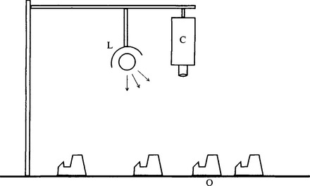
Figure 27.1 Simple arrangement for image acquisition: C, camera; L, light with simple reflector; O, objects on worktable or conveyor.
Even in this apparently simple case—one point light source and one camera—the situation can become quite complex. However, (5) is normally a reasonably marginal effect and is ignored in what follows. In addition, effect (3) can often be ignored except in one or two small regions of the image where sharply curved pieces of metal give rise to glints. This still leaves considerable scope for complication due to factors (1), (2), and (4).
Two important reasons may be cited for viewing the surfaces of objects. The first is when we wish to locate objects and their facets, and the second is when we wish to scrutinize the surfaces themselves. In the first instance, it is important to try to highlight the facets by arranging that they are lit differently, so that their edges stand out clearly. In the second instance, it might be preferable to do the opposite—that is, to arrange that the surfaces are lit very similarly, so that any variations in reflectivity caused by defects or blemishes stand out plainly. The existence of effects (1) and (2) implies that it is difficult to achieve both of these effects at the same time: one set of lighting conditions is required for optimum segmentation and location, and another set for optimum surface scrutiny. In most of this book, object location has been regarded as the more difficult task and therefore the one that needs the most attention. Hence, we have imagined that the lighting scheme is set up for this purpose. In principle, a point source of light is well adapted to this situation. However, it is easy to see that if a very diffuse lighting source is employed, then angles of incidence will tend to average out and effect (2) will dominate over (1) so that, to a first approximation, the observed brightness values will represent variations in surface reflectance. “Soft” or diffuse lighting also subdues specular reflections (effect (3)), so that for the most part they can be ignored.
Returning to the case of a single point source, recall (effect (4)) that shadows can become important. One special case when this is not so is when the light is projected from exactly the same direction as the camera. We return to this case later in this chapter. Shadows are a persistent cause of complications in image analysis. One problem is that it is not a trivial task to identify them, so they merely contribute to the overall complexity of any image and in particular add to the number of edges that have to be examined in order to find objects. They also make it much more difficult to use simple thresholding. (However, note that shadows can sometimes provide information that is of vital help in interpreting complex 3-D images—see, for example, Section 16.6.)
27.2.1 Eliminating Shadows
The above considerations suggest that it would be highly convenient if shadows could be eliminated. A strategy for achieving this elimination is to lower their contrast by using several light sources. Then the region of shadow from one source will be a region of illumination from another, and shadow contrast will be lowered dramatically. Indeed, if there are n lights, many positions of shadow will be illuminated by n– 1 lights, and their contrast will be so low that they can be eliminated by straightforward thresholding operations. However, if objects have sharp corners or concavities, there may still be small regions of shadow that are illuminated by only one light or perhaps no light at all. These regions will be immediately around the objects, and if the objects appear dark on a light background, shadows could make the objects appear enlarged, or cause shadow lines immediately around them. For light objects on a dark background this is normally less of a problem.
It seems best to aim for large numbers of lights so as to make the shadows more diffuse and less contrasting, and in the limit it appears that we are heading for the situation of soft lighting discussed earlier. However, this is not quite so. What is often required is a form of diffuse lighting that is still directional—as in the case of a diffuse source of restricted extent directly overhead. This can be provided very conveniently by a continuous ring light around the camera. This technique is found to eliminate shadows highly effectively, while retaining sufficient directionality to permit a good measure of segmentation of object facets to be achieved. That is, it is an excellent compromise, although it is certainly not ideal. For these reasons it is worth describing its effects in some detail. In fact, it is clear that it will lead to good segmentation of facets whose boundaries lie in horizontal planes but to poor segmentation of those whose boundaries lie in vertical planes.
The situation just described is very useful for analyzing the shape profiles of objects with cylindrical symmetry. The case shown in Fig. 27.2 involves a special type of chocolate biscuit with jam underneath the chocolate. If this is illuminated by a continuous ring light fairly high overhead (the proper working position), the region of chocolate above the edge of the jam reflects the light obliquely and appears darker than the remainder of the chocolate. On the contrary, if the ring light is lowered to near the worktable, the region above the edge of the jam appears brighter than the rest of the chocolate because it scatters light upward rather than sideways. There is also a particular height at which the ring light can make the jam boundary disappear (Fig. 27.3), this height being dictated by the various angles of incidence and reflection and by the relative direction of the ring light.2 In comparison, if the lighting were made completely diffuse, these effects would tend to disappear and the jam boundary would always have very low contrast.
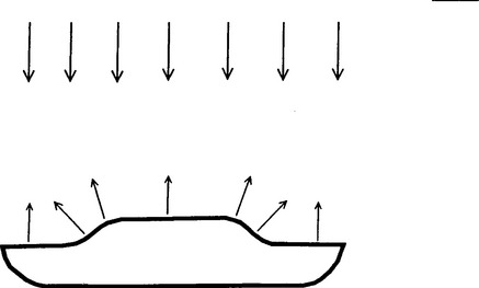
Figure 27.2 Illumination of a chocolate-and-jam biscuit. This figure shows the cross section of a particular type of round chocolate biscuit with jam underneath the chocolate. The arrows show how light arriving from vertically overhead is scattered by the various parts of the biscuit.
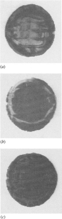
Figure 27.3 Appearance of the chocolate-and-jam biscuit of Fig. 27.2: (a) how the biscuit appears to a camera directly overhead when illuminated as in Fig. 27.2; (b) appearance when the lights are lowered to just above table level; (c) appearance when the lights are raised to an intermediate level making the presence of the jam scarcely detectable.
Suitable fluorescent ring lights are readily available and straightforward to use and provide a solution that is more practicable than the alternative means of eliminating shadows mentioned above—that of illuminating objects directly from the camera direction, for example, via a half-silvered mirror.
Earlier, the one case we did not completely solve arose when we were attempting to segment facets whose joining edges were in vertical planes. There appears to be no simple way of achieving a solution to this problem without recourse to switched lights (see Chapter 16). This matter is not discussed further here.
We have now identified various practical forms of lighting that can be used to highlight various object features and that eliminate complications as far as possible. These types of lighting are restricted in what they can achieve (as would clearly be expected from the shape-from-shading ideas of Chapter 16). However, they are exceedingly useful in a variety of applications. A final problem is that two lighting schemes may have to be used in turn, the first for locating objects and the second for inspecting their surfaces. However, this problem can largely be overcome by not treating the latter case as a special one requiring its own lighting scheme, but rather noting the direction of lighting and allowing for the resulting variation in brightness values by taking account of the known shape of the object. The opposite approach is generally of little use unless other means are used for locating the object. However, the latter situation frequently arises in practice. Imagine that a slab of concrete or a plate of steel is to be inspected for defects. In that case, the position of the object is known, and it is clearly best to set up the most uniform lighting arrangement possible, so as to be most sensitive to small variations in brightness at blemishes. This is, then, an important practical problem, to which we now turn.
27.2.2 Principles for Producing Regions of Uniform Illumination
While initially it may seem necessary to illuminate a worktable or conveyor uniformly, a more considered view is that a uniform flat material should appear uniform, so that the spatial distribution of the light emanating from its surface is uniform. The relevant quantity to be controlled is therefore the radiance of the surface (light intensity in the image). Following the work of Section 16.4 relating to Lambertian (matte) surfaces, the overall reflectance R of the surface is given by:
where R0 is the absolute reflectance of the surface and n, s are, respectively, unit vectors along the local normal to the surface and the direction of the light source.
The assumption of a Lambertian surface can be questioned, since most materials will give a small degree of specular reflection, but in this section we are interested mainly in those nonshiny substances for which equation (27.1) is a good approximation. In any case, special provision normally has to be made for examining surfaces with a significant specular reflectance component. However, notice that the continuous strip lighting systems considered below have the desirable property of largely suppressing any specular components.
Next we recognize that illumination will normally be provided by a set of lights at a certain height h above a worktable or conveyor. We start by taking the case of a single point source at height h. Supposing that this is displaced laterally through a distance a, so that the actual distance from the source to the point of interest on the worktable is d, I will have the general form:
where c is a constant factor (see Fig. 27.4).
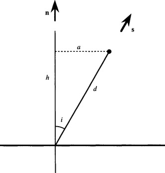
Figure 27.4 Geometry for a single point source illuminating a surface. Here a point light source at a height h above a surface illuminates a general point with angle of incidence i. n and s are, respectively, unit vectors along the local normal to the surface and the direction of the light source.
Equation (27.2) represents a distinctly nonuniform region of intensity over the surface. However, this problem may be tackled by providing a suitable distribution of lights. A neat solution is provided by a symmetrical arrangement of two strip lights that will help to make the reflected intensity much more uniform (Fig. 27.5). We illustrate this idea by reference to the well-known arrangement of a pair of Helmholtz coils—widely used for providing a uniform magnetic field, with the separation of the coils made equal to their radius so as to eliminate the second-order variation in field intensity. (Note that in a symmetrical arrangement of coils, all odd orders vanish, and a single dimensional parameter can be used to cancel the second order term.)
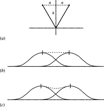
Figure 27.5 Effect of using two strip lights for illuminating a surface. (a) shows two strip lights at a height h above a surface, and (b) shows the resulting intensity patterns for each of the lights. The dotted line shows the combined intensity pattern. (c) shows the corresponding patterns when the separation of the lights is increased slightly.
In a similar way, the separation of the strip lights can be adjusted so that the second-order term vanishes (Fig. 27.5b). There is an immediate analogy also with the second-order Butterworth low-pass filter, which gives a maximally flat response, the second-order term in the frequency response curve being made zero, and the lowest order term then being the fourth-order term (Kuo, 1966). The last example demonstrates how the method might be improved further—by aiming for a Chebychev type of response in which there is some ripple in the pass band, yet the overall pass-band response is flatter (Kuo, 1966). In a lighting application, we should aim to start with the strip lights not just far enough apart so that the second-order term vanishes, but slightly further apart, so that the intensity is almost uniform over a rather larger region (Fig. 27.5c). This demonstrates that in practice the prime aim will be to achieve a given degree of uniformity over the maximum possible size of region.
In principle, it is easy to achieve a given degree of uniformity over a larger region by starting with a given response and increasing the linear dimensions of the whole lighting system proportionately. Though valid in principle, this approach will frequently be difficult to apply in practice. For example, it will be limited by convenience and by availability of the strip lights. It must also be noted that as the size of the lighting system increases, so must the power of the lights. Hence in the end we will have only one adjustable geometric parameter by which to optimize the response.
Finally, note that in most practical situations, it will be less useful to have a long narrow working region than one whose aspect ratio is close to unity. We shall consider two such cases—a circular ring light and a square ring light. The first of these is conveniently provided in diameters of up to at least 30 cm by commercially available fluorescent tubes, while the second can readily be constructed—if necessary on a much larger scale—by assembling a set of four linear fluorescent tubes. In this case we take the tubes to be finite in length, and in contact at their ends, the whole being made into an assembly that can be raised or lowered to optimize the system. Thus, these two cases have fixed linear dimensions characterized in each case by the parameter a, and it is h that is adjusted rather than a. To make comparisons easier, we assume in all cases that a is the constant and h is the optimization parameter (Fig. 27.6).
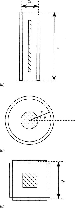
Figure 27.6 Lighting arrangements for obtaining uniform intensity. This diagram shows three arrangements of tubular lights for providing uniform intensity over fairly large regions, shown cross-hatched in each case. (a) shows two long parallel strip lights, (b) shows a circular ring light, and (c) shows four strip lights arranged to form a square “ring.” In each case, height h above the worktable must also be specified.
27.2.3 Case of Two Infinite Parallel Strip Lights
First we take the case of two infinite parallel strip lights. In this case, the intensity I is given by the sum of the intensities I1, I2 for the two tubes:
Suitable substitutions permit equation (27.3) to be integrated, and the final result is:
Differentiating I twice and setting d2I/dx2 = 0 at x = 0 eventually (Davies, 1997c) yield the maximally flat condition:
However, as noted earlier, it should be better to aim for minimum overall ripple over a region 0 ≤ x ≤ x1. The situation is shown in Fig. 27.7. We take the ripple ΔI as the difference in height between the maximum intensity Im and the minimum intensity I0, at x = 0, and on this basis the maximum permissible deviation in x is the value of x where the curve again crosses the minimum value I0.
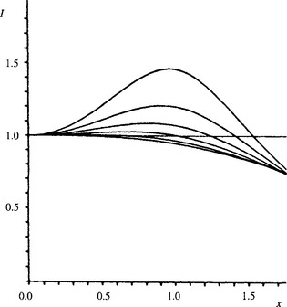
Figure 27.7 Intensity variation for two infinite parallel strip lights. This diagram shows the intensity variation I as a function of the distance x from the center of symmetry for six different values of h. h increases in steps of 0.2 from 0.8 for the top curve to 1.8 for the bottom curve. The value of h corresponding to the maximally flat condition is h = 1.732. x and h are expressed in units of a, while I is normalized to give a value of unity at x = 0.
A simple calculation shows that the intensity is again equal to I0 for x = x1, where
the graph of h versus x1 being the circle x2 + h2 = 3a2 (Fig. 27.8, top curve). It is interesting that the maximally flat condition is a special case of the new one, applying where x1 = 0.
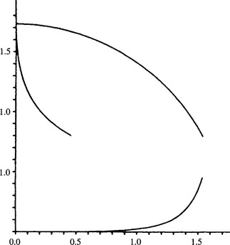
Figure 27.8 Design graphs for two parallel strip lights. Top, h v. x1. Left, h v. ΔI. Bottom, ΔI v. x1. The information in these graphs has been extracted from Fig. 27.7. In design work, a suitable compromise working position would be selected on the bottom curve, and then h would be determined from one of the other two curves. In practice, ΔI is the controlling parameter, so the left and bottom curves are the important ones, the top curve containing no completely new information.
Further mathematical analysis of this case is difficult; numerical computation leads to the graphs of Fig. 27.8. The top curve in Fig. 27.8 has already been referred to and shows the optimum height for selected ranges of values of x up to x1. Taken on its own, this curve would be valueless as the accompanying nonuniformity in intensity would not be known. This information is provided by the left curve in Fig. 27.8. However, for design purposes it is most important first to establish what range of intensities accompanies a given range of values of x, since this information (Fig. 27.8, bottom curve) will permit the necessary compromise between these variables to be made. Having decided on particular values of x1 and ΔI, the value of the optimization parameter h can then be determined from one of the other two graphs. Both are provided for convenience of reference. (It will be seen that once two of the graphs are provided, the third gives no completely new information.) Maximum acceptable variations in ΔI are assumed to be in the region of 20%, though the plotted variations are taken up to ∼50% to give a more complete picture. On the other hand, in most of the practical applications envisaged here, ΔI would be expected not to exceed 2 to 3% if accurate measurements of products are to be made.
The ΔI v. x1 variation varies faster than the fourth power of x1, there being a very sharp rise in ΔI for higher values of x1. This means that once ΔI has been specified for the particular application, little is to be gained by trying to squeeze extra functionality through going to higher values of x1, that is, in practice ΔI is the controlling parameter.
In the case of a circular ring light, the mathematics is more tedious (Davies, 1997c) and it is not profitable to examine it here. The final results are very similar to those for parallel strip lights. They would be used for design in the identical manner to that outlined earlier for the previous case.
In the case of a square ring light, the mathematics is again tedious (Davies, 1997c), but the results follow the same pattern and warrant no special comment.
27.2.4 Overview of the Uniform Illumination Scenario
Previous work on optical inspection systems has largely ignored the design of optimal lighting schemes. This section has tackled the problem in a particular case of interest—how to construct an optical system that makes a uniform matte surface appear uniformly bright, so that blemishes and defects can readily be detected with minimal additional computation. Three cases for which calculations have been carried out cover a good proportion of practical lighting schemes, and the design principles described here should be applicable to most other schemes that could be employed.
The results are best presented in the form of graphs. In any one case, the graph shows the tradeoff between variation in intensity and range of position on the working surface, from which a suitable working compromise can be selected. The other two graphs provide data for determining the optimization parameter (the height of the lights above the working surface).
A wide variety of lighting arrangements are compatible with the general principles presented above. Thus, it is not worthwhile to give any detailed dimensional specifications—especially as the lights might be highly directional rather than approximating to point or line sources. However, it is worth underlining that adjustment of just one parameter (the height) permits uniform illumination to be achieved over a reasonable region. Note that (as for a Chebyshev filter) it may be better to arrange a slightly less uniform brightness over a larger region than absolutely uniform brightness over a small region (as is achieved by exact cancellation of the second spatial derivatives of intensity). It is left to empirical tests to finalize the details of the design.
Finally, it should be reiterated that such a lighting scheme is likely to be virtually useless for segmenting object facets from each other—or even for discerning relatively low curvatures on the surface of objects. Its particular value lies in the scrutiny of surfaces via their absolute reflectivities, without the encumbrance of switched lights (see Chapter 16). It should also be emphasized that the aim of the discussion in the past few sections has been to achieve as much as possible with a simple static lighting scheme set up systematically. Naturally, such solutions are compromises, and again are no substitute for the full rigor of switched lighting schemes.
27.2.5 Use of Line-scan Cameras
Throughout this discussion it has been assumed implicitly that a conventional “area” camera is employed to view the objects on a worktable. However, when products are being manufactured in a factory they are frequently moved from one stage to another on a conveyor. Stopping the conveyor to acquire an image for inspection would impose unwanted design problems. For this reason use is made of the fact that the speed of the conveyor is reasonably uniform, and an area image is built up by taking successive linear snapshots. This is achieved with a line-scan camera that consists of a row of photocells on a single integrated circuit sensor. The orientation of the line of photocells must, of course, be normal to the direction of motion. More will be said later about the internal design of line-scan and other cameras. However, here we concentrate on the lighting arrangement to be used with such a camera.
When using a line-scan camera it is natural to select a lighting scheme that embodies the same symmetry as the camera. Indeed, the most obvious such scheme is a pair of long fluorescent tubes parallel to the line of the camera (and perpendicular to the motion of the conveyor). We caution against this “obvious” scheme, since a small round object (for example) will not be lit symmetrically. Of course, there are difficulties in considering this problem in that different parts of the object are viewed by the line-scan camera at different moments, but for small objects a linear lighting scheme will not be isotropic. This could lead to small distortions being introduced in measurements of object dimensions. This means that in practice the ring and other symmetrical lighting schemes described above are likely to be more closely optimal even when a line-scan camera is used. For larger objects, much the same situation applies, although the geometry is more complex to work out in detail.
Finally, the comment above that conveyor speeds are “reasonably uniform” should be qualified. The author has come across cases where this is true only as a first approximation. As with many mechanical systems, conveyor motion can be unreliable. For example, it can be jerky, and in extreme cases not even purely longitudinal! Such circumstances frequently arise through a variety of problems that cause slippage relative to the driving rollers—the effects of wear or of an irregular join in the conveyor material, misalignment of the driving rollers, and so on. Furthermore, the motors controlling the rollers may not operate at constant speed, either in the short term (e.g., because of varying load) or in the longer term (e.g., because of varying mains frequency and voltage). While, therefore, it cannot be assumed that a conveyor will operate in an ideal way, careful mechanical design can minimize these problems. However, when high accuracy is required, it will be necessary to monitor the conveyor speed, perhaps by using the optically coded disc devices that are now widely available, and feeding appropriate distance marker pulses to the controlling computer. Even with this method, it will be difficult to match in the longitudinal direction the extremely high accuracy3 available from the line-scan camera in the lateral direction. However, images of 512 × 512 pixels that are within 1 pixel accuracy in each direction should normally be available.
27.3 Cameras and Digitization
For many years the camera that was normally used for image acquisition was the TV camera with a vidicon or related type of vacuum tube. The scanning arrangements of such cameras became standardized, first to 405 lines, and later to 625 lines (or 525 lines in the United States). In addition, it is usual to interlace the image—that is, to scan odd lines in one frame and even lines in the next frame, then repeat the process, each full scan taking 1/25 second (1/30 second in the United States). There are also standardized means for synchronizing cameras and monitors, using line and frame “sync” pulses. Thus, the vacuum TV camera left a legacy of scanning techniques that are in the process of being eliminated with the advent of digital TV.4 However, as the result of the legacy is still present, it is worth including a few more details here.
The output of these early cameras is inherently analog, consisting of a continuous voltage variation, although this applies only along the line direction. The scanning action is discrete in that lines are used, making the output of the camera part analog and part digital. Hence, before the image is available as a set of discrete pixels, the analog waveform has to be sampled. Since some of the line scanning time is taken up with frame synchronization pulses, only about 550 lines are available for actual picture content. In addition, the aspect ratio of a standard TV image is 4:3 and it is common to digitize TV pictures as 512 × 768 or as 512 × 512 pixels. Note, too, that after the analog waveform has been sampled and pixel intensity values have been established, it is still necessary to digitize the intensity values.
Modern solid-state cameras are much more compact and robust and generate less noise. A very important additional advantage is that they are not susceptible to distortion,5 because the pixel pattern is fabricated very accurately by the usual integrated circuit photolithography techniques. They have thus replaced vacuum tube cameras in all except special situations.
Most solid-state cameras currently available are of the self-scanned CCD type; therefore, attention is concentrated on these in what follows. In a solid-state CCD camera, the target is a piece of silicon semiconductor that possesses an array of photocells at the pixel positions. Hence, this type of camera digitizes the image from the outset, although in one respect—that signal amplitude represents light intensity—the image is still analog. The analog voltages (or, more accurately, the charges) representing the intensities are systematically passed along analog shift registers to the output of the instrument, where they may be digitized to give 6 to 8 bits of gray-scale information (the main limitation here being lack of uniformity among the photosensors rather than noise per se).
The scanning arrangement of a basic CCD camera is not fixed, being fired at any desired rate by externally applied pulses. CCD cameras have been introduced which simulate the old TV cameras, with their line and frame sync pulses. In such cases, the camera initially digitizes the image into pixels, and these are shifted in the standard way to an output connector, being passed en route through a low-pass filter in order to remove the pixellation. When the resulting image is presented on a TV monitor, it appears exactly like a normal TV picture. Some problems are occasionally noticeable, however, when the depixellated image is resampled by a new digitizer for use in a computer frame store. Such problems are due to interference or beating between the two horizontal sampling rates to which the information has been subjected, and take the form of faint vertical lines. Although more effective low-pass filters should permit these problems to be eliminated, the whole problem is being eliminated by memory mapping of CCD cameras to bypass the analog legacy completely.
Another important problem relating to cameras is that of color response. The tube of the vacuum TV camera has a spectral response curve that peaks at much the same position as the spectral pattern of (“daylight”) fluorescent lights—which itself matches the response of the human eye (Table 27.1). However, CCD cameras have significantly lower response to the spectral pattern of fluorescent tubes (Table 27.1). In general, this may not matter too greatly, but when objects are moving, the integration time of the camera is limited and sensitivity can suffer. In such cases, the spectral response is an important factor and may dictate against use of fluorescent lights. (This is particularly relevant where CCD line-scan cameras are used with fast-moving conveyors.)
| Device | Band (nm) | Peak (nm) |
|---|---|---|
| Vidicon | 200–800 | ~550 |
| CCD | 400–1000 | ~800 |
| Fluorescent tube | 400–700 | ~600 |
| Human eye | 400–700 | ~550 |
In this table, the response of the human eye is included for reference. Note that the CCD response peaks at a much higher wavelength than the vidicon or fluorescent tube, and therefore is often at a disadvantage when used in conjunction with the fluorescent tube.
An important factor in the choice of cameras is the delay lag that occurs before a signal disappears and causes problems with moving images. Fortunately, the effect is entirely eliminated with the CCD camera, since the action of reading an image wipes the old image. However, moving images require frequent reading, and this implies loss of integration time and therefore loss of sensitivity—a factor that normally has to be made up by increasing the power of illuminating sources. Camera “burn-in” is another effect that is absent with CCD cameras but that causes severe problems with certain types of conventional cameras. It is the long-term retention of picture highlights in the light-sensitive material that makes it necessary to protect the camera against bright lights and to take care to make use of lens covers whenever possible. Finally, blooming is the continued generation of electron-hole pairs even when the light-sensitive material is locally saturated with carriers, with the result that the charge spreads and causes highlights to envelop adjacent regions of the image. Both CCD and conventional camera tubes are subject to this problem, although it is inherently worse for CCDs. This has led to the production of antiblooming structures in these devices: space precludes detailed discussion of the situation here.
27.3.1 Digitization
Digitization is the conversion of the original analog signals into digital form. There are many types of analog-to-digital converters (ADCs), but the ones used for digitizing images have so much data to process—usually in a very short time if realtime analysis is called for—that special types have to be employed. The only one considered here is the “flash” ADC, so called because it digitizes all bits simultaneously, in a flash. It possesses n–1 analog comparators to separate n gray levels, followed by a priority encoder to convert the n–1 results into normal binary code. Such devices produce a result in a very few nanoseconds and their specifications are generally quoted in megasamples per second (typically in the range 50–200 megasamples/second). For some years these were available only in 6-bit versions (apart from some very expensive parts), but today it is possible to obtain 8-bit versions at almost negligible cost.6 Such 8-bit devices are probably sufficient for most needs considering that a certain amount of sensor noise, or variability, is usually present below these levels and that it is difficult to engineer lighting to this accuracy.
27.4 The Sampling Theorem
The Nyquist sampling theorem underlies all situations where continuous signals are sampled and is especially important where patterns are to be digitized and analyzed by computers. This makes it highly relevant both with visual patterns and with acoustic waveforms. Hence, it is described briefly in this section.
Consider the sampling theorem first in respect of a 1-D time-varying waveform. The theorem states that a sequence of samples (Fig. 27.9) of such a waveform contains all the original information and can be used to regenerate the original waveform exactly, but only if (1) the bandwidth W of the original waveform is restricted and (2) the rate of sampling f is at least twice the bandwidth of the original waveform—that is, f ≥ 2W. Assuming that samples are taken every T seconds, this means that 1/T ≥ 2W.
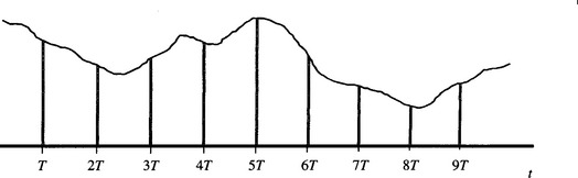
Figure 27.9 The process of sampling a time-varying signal. A continuous time-varying 1-D signal is sampled by narrow sampling pulses at a regular rate fr = 1/T, which must be at least twice the bandwidth of the signal.
At first, it may be somewhat surprising that the original waveform can be reconstructed exactly from a set of discrete samples. However, the two conditions for achieving perfect reconstruction are very stringent. What they are demanding in effect is that the signal must not be permitted to change unpredictably (i.e., at too fast a rate) or else accurate interpolation between the samples will not prove possible (the errors that arise from this source are called “aliasing” errors).
Unfortunately, the first condition is virtually unrealizable, since it is nearly impossible to devise a low-pass filter with a perfect cutoff. Recall from Chapter 3 that a low-pass filter with a perfect cutoff will have infinite extent in the time domain, so any attempt at achieving the same effect by time domain operations must be doomed to failure. However, acceptable approximations can be achieved by allowing a “guard-band” between the desired and actual cutoff frequencies. This means that the sampling rate must therefore be higher than the Nyquist rate. (In telecommunications, satisfactory operation can generally be achieved at sampling rates around 20% above the Nyquist rate—see Brown and Glazier, 1974.)
One way to recover the original waveform is to apply a low-pass filter. This approach is intuitively correct because it acts in such a way as to broaden the narrow discrete samples until they coalesce and sum to give a continuous waveform. This method acts in such a way as to eliminate the “repeated” spectra in the transform of the original sampled waveform (Fig. 27.10). This in itself shows why the original waveform has to be narrow-banded before sampling—so that the repeated and basic spectra of the waveform do not cross over each other and become impossible to separate with a low-pass filter. The idea may be taken further because the Fourier transform of a square cutoff filter is the sinc (sin u/u) function (Fig. 27.11). Hence, the original waveform may be recovered by convolving the samples with the sinc function (which in this case means replacing them by sinc functions of corresponding amplitudes). This broadens out the samples as required, until the original waveform is recovered.
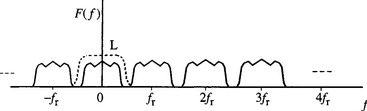
Figure 27.10 Effect of low-pass filtering to eliminate repeated spectra in the frequency domain f r, sampling rate; L, low-pass filter characteristic). This diagram shows the repeated spectra of the frequency transform F(f) of the original sampled waveform. It also demonstrates how a low-pass filter can be expected to eliminate the repeated spectra to recover the original waveform.
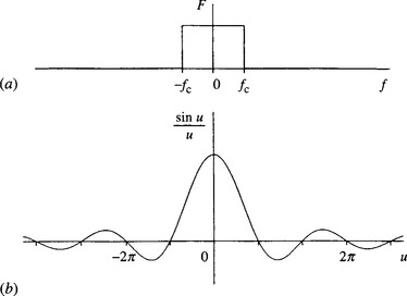
Figure 27.11 The sinc (sin u/u) function shown in (b) is the Fourier transform of a square pulse (a) corresponding to an ideal low-pass filter. In this case, u = 2πfct, fc being the cutoff frequency.
So far we have considered the situation only for 1-D time-varying signals. However, recalling that an exact mathematical correspondence exists between time and frequency domain signals on the one hand and spatial and spatial frequency signals on the other, the above ideas may all be applied immediately to each dimension of an image (although the condition for accurate sampling now becomes 1/X ≥ 2WX, where X is the spatial sampling period and WX is the spatial bandwidth). Here we accept this correspondence without further discussion and proceed to apply the sampling theorem to image acquisition.
Consider next how the signal from a TV camera may be sampled rigorously according to the sampling theorem. First, it is plain that the analog voltage comprising the time-varying line signals must be narrow-banded, for example, by a conventional electronic low-pass filter. However, how are the images to be narrow-banded in the vertical direction? The same question clearly applies for both directions with a solid-state area camera. Initially, the most obvious solution to this problem is to perform the process optically, perhaps by defocussing the lens. However, the optical transform function for this case is frequently (i.e., for extreme cases of defocusing) very odd, going negative for some spatial frequencies and causing contrast reversals; hence, this solution is far from ideal (Pratt, 2001). Alternatively, we could use a diffraction-limited optical system or perhaps pass the focused beam through some sort of patterned or frosted glass to reduce the spatial bandwidth artificially. None of these techniques will be particularly easy to apply nor will accurate solutions be likely to result. However, this problem is not as serious as might be imagined. If the sensing region of the camera (per pixel) is reasonably large, and close to the size of a pixel, then the averaging inherent in obtaining the pixel intensities will in fact perform the necessary narrow-banding (Fig. 27.12). To analyze the situation in more detail, note that a pixel is essentially square with a sharp cutoff at its borders. Thus, its spatial frequency pattern is a 2-D sinc function, which (taking the central positive peak) approximates to a low-pass spatial frequency filter. This approximation improves somewhat as the border between pixels becomes fuzzier.
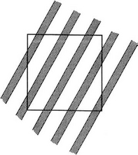
Figure 27.12 Low-pass filtering carried out by averaging over the pixel region. An image with local high-frequency banding is to be averaged over the whole pixel region by the action of the sensing device.
The point here is that the worst case from the point of view of the sampling theorem is that of extremely narrow discrete samples, but this worst case is unlikely to occur with most cameras. However, this does not mean that sampling is automatically ideal—and indeed it is not, since the spatial frequency pattern for a sharply defined pixel shape has (in principle) infinite extent in the spatial frequency domain. The review by Pratt (2001) clarifies the situation and shows that there is a tradeoff between aliasing and resolution error. Overall, it is underlined here that quality of sampling will be one of the limiting factors if one aims for the greatest precision in image measurement. If the bandwidth of the presampling filter is too low, resolution will be lost; if it is too high, aliasing distortions will creep in; and if its spatial frequency response curve is not suitably smooth, a guard band will have to be included and performance will again suffer.
27.5 Concluding Remarks
This chapter has sought to give some background to the problems of acquiring images, particularly for inspection applications. Methods of illumination were deemed to be worthy of considerable attention since they furnish means by which the practitioner can help to ensure that an inspection system operates successfully—and indeed that its vision algorithms are not unnecessarily complex, thereby necessitating excessive hardware expense for real-time implementation. Means of arranging reasonably uniform illumination and freedom from shadows have been taken to be of significant relevance and are allotted fair attention. (It is of interest that these topics are scarcely mentioned in most books on this subject—a surprising fact that perhaps indicates the importance that most authors ascribe to this vital aspect of the work.) For recent publications on illumination and shadow elimination, see Section 27.6.
By contrast, camera systems and digitization techniques have been taken to be purely technical matters to which little space could be devoted. (To be really useful—and considering that most workers in this area buy commercial cameras and associated frame-grabbing devices ready to plug into a variety of computers—whole chapters would have been required for each of these topics.) Because of its theoretical importance, it appeared to be relevant to give some background to the sampling theorem and its implications, although, considering the applications covered in this book, further space devoted to this topic did not appear to be justified (see Rosie, 1966 and Pratt, 2001 for more details).
Computer vision systems are commonly highly dependent on the quality of the incoming images. This chapter has shown that image acquisition can often be improved, particularly for inspection applications, by arranging regions of nearly uniform illumination, so that shadows and glints are suppressed, and the vision algorithms are much simplified and speeded up.
27.6 Bibliographical and Historical Notes
It is regrettable that very few papers and books give details of lighting schemes that are used for image acquisition, and even fewer give any rationale or background theory for such schemes. Hence, some of the present chapter appears to have broken new ground in this area. However, Batchelor et al. (1985) and Browne and Norton-Wayne (1986) give much useful information on light sources, filters, lenses, light guides, and so on, thereby complementing the work of this chapter. (Indeed, Batchelor et al. (1985) give a wealth of detail on how unusual inspection tasks, such as those involving internal threads, may be carried out.)
Details of various types of scanning systems, camera tubes, and solid-state (e.g., CCD) devices are widely available; see, for example, Biberman and Nudelman (1971), Beynon and Lamb (1980), Batchelor et al. (1985), Browne and Norton-Wayne (1986), and various manufacturers’ catalogs. Note that much of the existing CCD imaging device technology dates from the mid-1970s (Barbe, 1975; Weimer, 1975) and is still undergoing development.
Flash (bit-parallel) ADCs are by now used almost universally for digitizing pixel intensities. For a time TRW Inc. (a former USA company, now apparently merged with Northrup Grumman Corp.) was preeminent in this area, and the reader is referred to the catalog of this and other electronics manufacturers for details of these devices.
The sampling theorem is well covered in numerous books on signal processing (see, for example, Rosie, 1966). However, details of how band-limiting should be carried out prior to sampling are not so readily available. Only a brief treatment is given in Section 27.4: for further details, the reader is referred to Pratt (2001) and to references contained therein.
The work of Section 27.2 arose from the author’s work on food product inspection, which required carefully controlled lighting to facilitate measurement, improve accuracy, and simplify (and thereby speed up) the inspection algorithms (Davies, 1997d). Similar motivation drove Yoon et al. (2002) to attempt to remove shadows by switching different lights on and off, and then using logic to eliminate the shadows. Under the right conditions, it was only necessary to find the maximum of the individual pixel intensities between the various images. However, in outdoor scenes it is difficult to control the lighting. Instead, various rules must be worked out for minimizing their effect. Prati et al. (2001) have done a comparative evaluation of available methods. Other work on shadow location and elimination has been reported by Rosin and Ellis (1995), Mikic et al. (2000), and Cucchiara et al. (2003). Finally, Koch et al. (2001) have presented results on the use of switched lights to maintain image intensity regardless of changes of ambient illumination and to limit the overall dynamic range of image intensities so that the risk of over- or underexposing the scene is drastically reduced.
1 Referring to equation (15.12), R0 is the absolute surface reflectivity and R1 is the specularity.
2 The latter two situations are described for interest only.
3 A number of line-scan cameras are now available with 4096 or greater numbers of photocells in a single linear array. In addition, these arrays are fabricated using very high-precision technology (see Section 27.3), so considerable reliance can be placed on the data they provide.
4 All the vestiges of the old system will not have been swept away until all TV receivers and monitors are digital as well as the cameras themselves.
5 However, this does not prevent distortions from being introduced by other mechanisms—poor optics, poor lighting arrangements, perspective effects, and so on.
6 Indeed, as is clear from the advent of cheap web cameras and digital cameras, it is becoming virtually impossible to get noncolor versions of such devices.