
CHAPTER 23 Inspection of Cereal Grains
23.1 Introduction
Cereal grains are among the most important of the foods we grow. A large proportion of cereal grains is milled and marketed as flour, which is then used to produce bread, cakes, biscuits, and many other commodities. Cereal grains can also be processed in a number of other ways (such as crushing), and thus they form the basis of many breakfast cereals. In addition, some cereal grains, or cereal kernels, are eaten with a minimum of processing. Rice is an obvious member of this category—though whole wheat and oat grains are also consumed as decorative additives to “granary” loaves.
Wheat, rice, and other cereal grains are shipped and stored in huge quantities measured in millions of tons, and a very large international trade exists to market these commodities. Transport also has to be arranged between farmers, millers, crushers, and the major bakers and marketers. Typically, transit by road or rail is in relatively small loads of up to twenty tons, and grain depots, warehouses, and ports are not unlikely to receive lorries containing such consignments at intervals ranging from 20 minutes to as little as 3 minutes. As a result of all the necessary transportation and storage, grains are subject to degradation, including damage, molds, sprouting, and insect infestation. In addition, because grains are grown on the land and threshed, potential contamination by rodent droppings, stones, mud, chaff, and foreign grains arises. Finally, the quality of grain from various sources will not be uniformly high, and varietal purity is an important concern.
These factors mean that, ideally, the grain that arrives at any depot should be inspected for many possible causes of degradation. This chapter is concerned with grain inspection. In the space of one chapter we cannot cover all possible methods and modes of inspection, especially since changes in this area are accelerating. Not only are inspection methods evolving rapidly, but so are the standards against which inspection is carried out. To some extent, the improvement of automatic inspection methods and the means of implementing them efficiently in hardware are helping to drive the process onward. We shall explore the situation with the aid of three main case studies, and then we shall look at the overall situation.
The first case study involves the examination of grains to locate rodent droppings and molds such as ergot; the second considers how grains may be scrutinized for insects such as the saw-toothed grain beetle; and the third deals with inspection of the grains themselves. However, this last case study will be more general and will concern itself less with scrutiny of individual grains than with how efficiently they can be located. This is an important factor when truckloads of grains are arriving at depots every few minutes—leading to the need to sample on the order of 300 grains per second. As observed in Chapter 22, object location can involve considerably more computation than object scrutiny and measurement.
23.2 Case Study 1: Location of Dark Contaminants in Cereals
Grain quality needs to be monitored before processing to produce flour, breakfast cereals, and myriad other derived products. So far, automated visual inspection has been applied mainly to the determination of grain quality (Ridgway and Chambers, 1996), with concentration on varietal purity (Zayas and Steele, 1990; Keefe, 1992) and the location of damaged grains (Liao et al., 1994). Relatively little attention has been paid to the detection of contaminants. There is the need for a cheap commercial system that can detect insect infestations and other important contaminants in grain, while not being confused by “permitted admixture” such as chaff and dust. (Up to ∼2% is normally permitted.) The inspection work described in this case study (Davies et al., 1998a) pays particular attention to the detection of certain important noninsect contaminants. Relevant contaminants in this category include rodent (especially rat and mouse) droppings, molds such as ergot, and foreign seeds. (Note that ergot is poisonous to humans, so locating any instances of it is of special importance.) In this case study, the substrate grain is wheat, and foreign seeds such as rape would be problematic if present in too great a concentration.
Many of the potential contaminants for wheat grains (and for grains of similar general appearance such as barley or oats) are quite dark in color. This means that thresholding is the most obvious approach for locating them. However, a number of problems arise in that shadows between grains, dark patches on the grains, chaff, and other admixture components, together with rapeseeds, appear as false alarms. Further recognition procedures must therefore be invoked to distinguish between the various possibilities. As a result, the thresholding approach is not as attractive as it might have a priori been thought (Fig. 23.1a, b). This problem is exacerbated by the extreme speed of processing required in real applications. For example, a successful device for monitoring truckloads of grain might well have to analyze a 3-kg sample of grain in three minutes (the typical time between arrival of lorries at a grain terminal), and this would correspond to some 60,000 grains having to be monitored for contaminants in that time. This places a distinct premium on rapid, accurate image analysis.
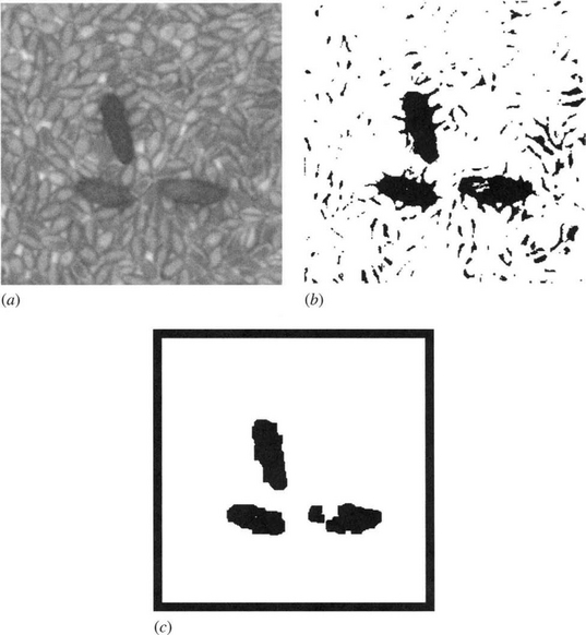
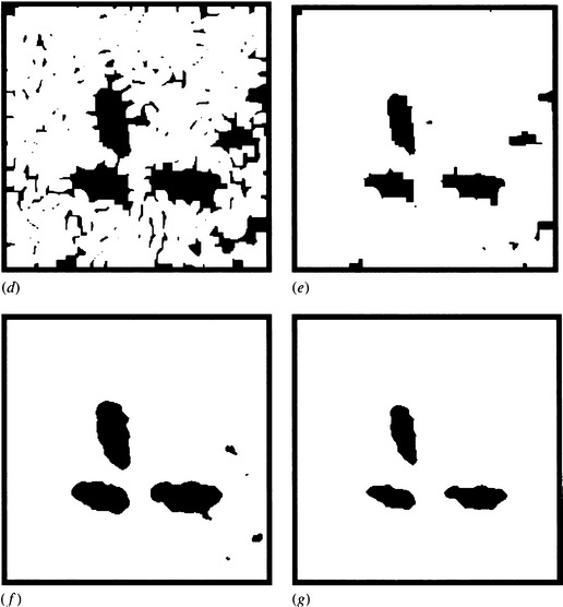
Figure 23.1 Effects of various operations and filters on a grain image. (a) Grain image containing several contaminants (rodent droppings). (b) Thresholded version of (a). (c) Result of erosion and dilation on (b). (d) Result of dilation and erosion on (b). (e) Result of erosion on (d). (f) Result of applying 11 × 11 median filter to (b). (g) Result of erosion on (f). In all cases, “erosion” means three applications of the basic 3 × 3 erosion operator, and similarly for “dilation.”
This case study concentrates on monitoring grain for rodent droppings. As already indicated, this type of contaminant is generally darker than the grain background, but it cannot simply be detected by thresholding since there are significant shadows between the grains, which themselves often have dark patches. In addition, the contaminants are speckled because of their inhomogeneous constitution and because of lighting and shadow effects. Despite these problems, human operators can identify the contaminants because they are relatively large and their shape follows a distinct pattern (e.g., an aspect ratio of three or four to one). Thus, the combination of size, shape, relative darkness, and speckle characterizes the contaminants and differentiates them from the grain substrate.
Designing efficient, rapidly operating algorithms to identify these contaminants presents a challenge, but an obvious way of meeting it, as we shall see in the next subsection, is via mathematical morphology.
23.2.1 Application of Morphological and Nonlinear Filters to Locate Rodent Droppings
The obvious approach to locating rodent droppings is to process thresholded images by erosion and dilation. (Erosion followed by dilation is normally termed opening, but we will not use that term here in order to retain the generality of not insisting on exactly the same number of erosion and dilation operations. In inspection it is the final recognition that must be emphasized rather than some idealized morphological process.) In this way, the erosions would eliminate shadows between grains and discoloration of grains, and the subsequent dilations would restore the shapes and sizes of the contaminants. The effect of this procedure is shown in Fig. 23.1c. Note that the method has been successful in eliminating the shadows between the grains but has been decidedly weak in coping with light regions on the contaminants. Remembering that although considerable uniformity might be expected between grains, the same cannot be said about rodent droppings, whose size, shape, and color vary quite markedly. Hence, the erosion–dilation schema has limited value, though it would probably be successful in most instances. Accordingly, other methods of analysis were sought (Davies et al., 1998a).
The second approach to locating rodent droppings is to compensate for the deficiency of the previous approach by ensuring that the contaminants are consolidated even if they are speckled or light in places. Thus, an attempt was made to apply dilation before erosion. The effect of this approach is shown in Fig. 23.1d. Notice that the result is to consolidate the shadows between grains even more than the shapes of the contaminants. Even when an additional few erosions are applied (Fig. 23.1e) the consolidated shadows do not disappear and are of comparable sizes to the contaminants. Overall, the approach is not viable, for it creates more problems than it solves. (The number of false positives far exceeds the number of false negatives, and similarly for the total areas of false positives and false negatives.) One possibility is to use the results of the earlier erosion–dilation schema as “seeds” to validate a subset of the dilation–erosion schema. However, this would be far more computation intensive, and the results would not be especially impressive (see Fig. 23.1c, e). Instead, a totally different approach was adopted.
The new approach was to apply a large median filter to the thresholded image, as shown in Fig. 23.1f. This gives good segmentation of the contaminants, retaining their intrinsic shape to a reasonable degree, and it suppresses the shadows between grains quite well. In fact, the shadows immediately around the contaminants enhance the sizes of the contaminants in the median filtered image, whereas some shadows further away are consolidated and retained by the median filtering. A reasonable solution is to perform a final erosion operation (Fig. 23.1g). This approach eliminates the extraneous shadows and brings the contaminants back to something like their proper size and shape; although the lengths are slightly curtailed, this is not a severe disadvantage. The median filtering–erosion schema easily gave the greatest fidelity to the original contaminants, while being particularly successful at eliminating other artifacts (Davies et al., 1998a).
Finally, although median filtering is intrinsically more computation intensive than erosion and dilation operations, many methods have been devised for accelerating median operations (see Chapter 3). Indeed, the speed aspect was found to be easily soluble within the specification set out above.
23.2.2 Appraisal of the Various Schemas
In the previous section, we showed that two basic schemas that aimed in the one case to consolidate the background and then the contaminants and in the other to consolidate the contaminants and then the background failed because each interfered with the alternate region. The median-based schema apparently avoided this problem because it was able to tackle both regions at once without prejudicing either. It is interesting to speculate that in this case the median filter is acting as an analytical device that carefully meditates and obtains the final result in a single rigorous stage, thereby avoiding the error propagation inherent in a two-stage process. Curiously, there seems to be no prior indication of this particular advantage of the median filter in the preexisting and rather wide morphological literature.
23.2.3 Problems with Closing
This case study required the use of a median filter coupled with a final erosion operation to eliminate artifacts in the background. An earlier test similarly involved a closing operation (a dilation followed by an erosion), followed by a final erosion. In other applications, grains or other small particles are often grouped by applying a closing operation to locate the regions where the particles are situated (Fig. 8.6). It is interesting to speculate whether, in the latter type of approach, closing should occasionally be followed by erosion, and also whether the final erosions used in our tests on grain were no more than ad hoc procedures or whether they were vital to achieve the defined goal.
Davies (2000c) analyzed the situation, which is summarized in Sections 8.6.1 and 8.6.2. The analysis starts by considering two regions containing small particles with occurrence densities ρ1, ρ2, where ρ1 > ρ2 (Figs. 8.7 and 8.8). It finds that a final erosion is indeed required to eliminate a shift in the region boundary, the estimated shift δ being1
where a is the radius of the dilation kernel and b is the width of the particles in region 2.
If b = 0, no shift will occur, but for particles of measurable size this is not so. If b is comparable to a or if a is much greater than 1, a substantial final erosion may be required. On the other hand, if b is small, the two-dimensional shift may be less than 1 pixel. In that case it will not be correctable by a subsequent erosion, though it should be remembered that a shift has occurred, and any corrections relating to the size of region 1 can be made during subsequent analysis. Although in this work the background artifacts were induced mainly by shadows around and between grains, in other cases impulse noise or light background texture could give similar effects. Care must be taken to select a morphological process that limits any overall shifts in region boundaries. In addition, the whole process can be modeled and the extent of any necessary final erosion can be estimated accurately. More particularly, the final erosion is a necessary measure and is not merely an ad hoc procedure (Davies, 2000c).
23.3 Case Study 2: Location of Insects
As noted in the first case study, a cheap commercial system that can detect a variety of contaminants in grain is needed. The present case study pays particular attention to the need to detect insects. Insects present an especially serious threat because they can multiply alarmingly in a short span of time, so greater certainty of detection is vital in this case. A highly discriminating method was therefore required for locating adult insects (Davies et al., 1998b).
Not surprisingly, thresholding initially seemed to be the approach that offered the greatest promise for locating insects, which appear dark relative to the light brown color of the grain. However, early tests on these lines showed that many false alarms would result from chaff and other permitted admixture, from less serious contaminants such as rapeseeds, and even from shadows between, and discolorations on, the grains themselves (Fig. 23.2). These considerations led to the use of the linear feature detection approach for detecting small adult insects. This proved possible because these insects appear as dark objects with a linear (essentially bar-shaped) structure. Hence, attempts to detect them by applying bar-shaped masks ultimately led to a linear feature detector that had good sensitivity for a reasonable range of insect sizes. Before proceeding, we consider the problems of designing linear feature detector masks.
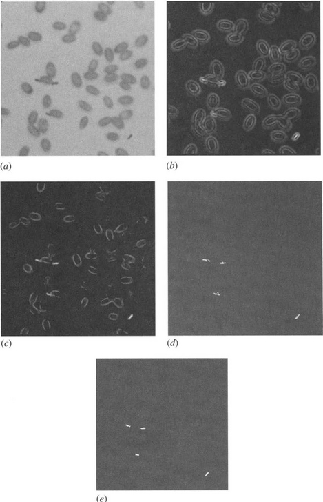
Figure 23.2 Insects located by line segment detector. (a) Original image. (b) Result of applying vectorial operator. (c) Result of masking (b) using an intensity threshold at a standard high level. (d) Result of thresholding (c). (e) Result of applying TM operation within (d).
23.3.1 The Vectorial Strategy for Linear Feature Detection
In earlier chapters we found that location of features in 3 × 3 windows typically required the application of eight template masks in order to cope with arbitrary orientation. In particular, to detect corners, eight masks were required, while only one was needed to locate small holes because of the high degree of symmetry present in the latter case (see Chapters 13 and Chapter 14). To detect edges by this means, four masks were required because 180° rotations correspond to a sign change that effectively eliminates the need for half of the masks. However, edge detection is a special case, for edges are vector quantities with magnitude and direction. Hence, they are fully definable using just two component masks. In contrast, a typical line segment detection mask would have the form:
This indicates that four masks are sufficient, the total number being cut from eight to four by the particular rotation symmetry of a line segment. Curiously, it has been shown that although only edges qualify as strict vectors, requiring just two component masks, the same can be made to apply for line segments. To achieve this, a rather unusual set of masks has to be employed:2
 (23.2)
The two masks are given different weights so that some account can be taken of the fact that the nonzero coefficients are, respectively, 1 and![]() pixels from the center pixel in the window. These masks give responses g0, g45 leading to:
pixels from the center pixel in the window. These masks give responses g0, g45 leading to:
where the additional factor of one-half in the orientation arises as the two masks correspond to basic orientations of 0° and 45° rather than 0° and 90° (Davies, 1997e). Nevertheless, these masks can cope with the full complement of orientations because line segments have 180° rotational symmetry and the final orientation should only be determined within the range 0° to 180°. In Section 23.5 we comment further on the obvious similarities and differences between equations (23.3), (23.4), and those pertaining to edge detection
Next, we have to select appropriate values of the coefficients A and B. Applying the above masks to a window with the intensity pattern

leads to the following responses at 0° and 45°:
Using this model, Davies (1997e) carried out detailed calculations for the case of a thin line of width w passing through the center of the 3 × 3 window, pixel responses being taken in proportion to the area of the line falling within each pixel. However, for lines of substantial width, theory proved intractable, and simulations were needed to determine the outcome. The remarkable aspect of the results was the high orientation accuracy that occurred for w = 1.4, in the case when B/A = 0.86, which gave a maximum error of just 0.4 °. In the following discussion, we will not be concerned with obtaining a high orientation accuracy, but will be content to use equation (23.3) in order to obtain an accurate estimate of line contrast using just two masks, thereby saving on computation. The reason for this is the need to attain high sensitivity in the detection of image features that correspond to insect contaminants rather than to pass results on to high-level interpretation algorithms, as orientation is not an important output parameter in this application.
23.3.2 Designing Linear Feature Detection Masks for Larger Windows
When larger windows are used, it is possible to design the masks more ideally to match the image features that have to be detected, because of the greater resolution then permitted. However, there are many more degrees of freedom in the design, and there is some uncertainty as to how to proceed. The basic principle (Davies et al., 1998b) is to use masks whose profile matches the intensity profile of a linear feature around a ring of radius R centered on the feature, and at the same time a profile that follows a particular mathematical model—namely, an approximately sinusoidal amplitude variation. For a given linear feature of width w, the sinusoidal model will achieve the best match for a thin ring of radius R0 for which the two arc lengths within the feature are each one quarter of the circumference 2πR0 of the ring. Simple geometry (Fig. 23.3) shows that this occurs when:
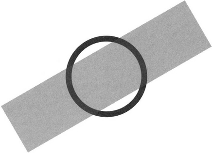
Figure 23.3 Geometry for application of a thin ring mask. Here two quarters of the ring mask lie within, and two outside, a rectangular bar feature.
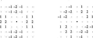
The width ΔR of the ring should in principle be infinitesimal, but in practice, considering noise and other variations in the dataset, ΔR can validly be up to about 40% of R0. The other relevant factor is the intensity profile of the ring, and how accurately this has to map to the intensity profile of the linear features that are to be located in the image. In many applications, such linear features will not have sharp edges but will be slightly fuzzy, and the sides will have significant and varying intensity gradient. Thus, the actual intensity profile is likely to correspond reasonably closely to a true sinusoidal variation. Masks designed on this basis proved close to optimal when experimental tests were made (Davies et al., 1998b). Figure 23.4 shows masks that resulted from this type of design process for one specific value of R (2.5 pixels).
23.3.3 Application to Cereal Inspection
The main class of insect targeted in this study (Davies et al., 1998b) was Oryzaephilus surinamensis (saw-toothed grain beetle). Insects in this class approximate to rectangular bars of about 10 × 3 pixels, and masks of size 7 × 7 (Fig. 23.4) proved to be appropriate for identifying the pixels on the centerlines of these insects. In addition, the insects could appear in any orientation, so potentially quite a large number of template masks might be required: this would have the disadvantage that their sequential implementation would be highly computation intensive and not conducive to real-time operation. Accordingly, it was natural to employ the vectorial approach to template matching, in which two orthogonal masks would be used as outlined above instead of the much larger number needed when using a more conventional approach.
Preliminary decisions on the presence of the insects were made by thresholding the output of the vectorial operator. However, the vectorial operator responses for insectlike bars have a low-intensity surround, which is joined to the central response at each end. Between the low-intensity surround and the central response, the signal drops close to zero except near the ends (Fig. 23.2b). This response pattern is readily understandable because symmetry demands that the signal be zero when the centers of the masks are coincident with the edge of the bar. To avoid problems from the parts of the response pattern outside the object, intensity thresholding (applied separately to the original image) was used to set the output to zero where it indicates no insect could be present (Fig. 23.2c). The threshold level was deliberately set high so as to avoid overdependence on this limited procedure.
23.3.4 Experimental Results
In laboratory tests, the vectorial operator was applied to 60 grain images containing a total of 150 insects. The output of the basic enhancement operator (described in Section 23.1) was thresholded to perform the actual detection and then passed to an area discrimination procedure. In accordance with our other work on grain images, objects having fewer than 6 pixels were eliminated, as experience had shown that these are most likely to be artifacts due, for example, to dark shadows or discolorations on the grains.
The detection threshold was then adjusted to minimize the total number of errors.3 This operation resulted in one false positive and three false negatives, so the great majority of the insects were detected. One of the false negatives was due to two insects that were in contact being interpreted as one. The other false negatives were due to insects being masked by lying along the edges of grains. The single false positive was due to the dark edge of a grain appearing (to the algorithm) similar to an insect.
Although adjustment of the detection threshold was found to eliminate either the false positive or two of the false negatives (but not the one in which two insects were in contact), the ultimate reason the total number of errors could not be reduced further lay in the limited sensitivity of the vectorial operator masks, which after all contain relatively few coefficients. This was verified by carrying out a test with a set of conventional template matching (TM) masks (Fig. 23.5), which led to a single false negative (due to the two insects being in contact) and no false positives—and a much increased computational load (Davies et al., 2003a). It was accepted that the case of two touching insects would remain a problem that could be eliminated only by introducing a greater level of image understanding—an aspect beyond the scope of this work (though curiously, the problem could easily be eliminated in this particular instance by noting the excessive length and/or area of this one object).
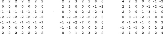
Figure 23.5 7 × 7 template matching masks. There are eight masks in all, oriented at multiples of 22.5° relative to the x-axis. Only three are shown because the others are straightforwardly generated by 90° rotation and reflection (symmetry) operations.
Next, it was desired to increase the interpretation accuracy of the vectorial operator in order to limit computation, and it seemed worth trying to devise a two-stage system, which would combine the speed of the vectorial operator with the accuracy of TM. Accordingly, the vectorial operator was used to create regions of interest for the TM operator. To obtain optimum performance, it was found necessary to decrease the vectorial operator threshold level to reduce the number of false negatives, leaving a slightly increased number of false positives that would subsequently be eliminated by the TM operator. The final result was an error rate exactly matching that of the TM operator, but a considerably reduced overall execution time composed of the adjusted vectorial operator execution time plus the TM execution time for the set of regions of interest. Further speed improvements, and no loss in accuracy, resulted from employing a dilation operation within the vectorial operator to recombine fragmented insects before applying the final TM operator. In this case, the vectorial operator was used without reducing its threshold value. At this stage, the speedup factor on the original TM operator was around seven (Davies et al., 2003a).
Finally, intensity thresholding was used as a preliminary skimming operation on the vectorial operator—where it produced a speedup by a factor of about 20. This brought the overall speedup factor on the original TM algorithm into the range 50–100, being close to 100 where insects are rare. Perhaps more important, the combined algorithm was in line with the target to inspect 3 kg of grain for a variety of contaminants within three minutes.
23.4 Case Study 3: High-speed Grain Location
As already mentioned, object location often requires considerable computation, for it involves unconstrained search over the image data. As a result, the whole process of automated inspection can be slowed down significantly, which can be of crucial importance in the design of real-time inspection systems. If the scrutiny of particular types of objects requires quite simple dimensional measurements to be made, the object location routine can be the bottleneck. This case study is concerned with the high-speed location of objects in 2-D images, a topic on which relatively little systematic work has been carried out—at least on the software side. Many studies have, however, been made on the design of hardware accelerators for image processing. Because hardware accelerators represent the more expensive option, this case study concentrates on software solutions to the problem and then specializes it to the case of cereal grains in images.
23.4.1 Extending an Earlier Sampling Approach
In an earlier project, Davies (1987l) addressed the problem of finding the centers of circular objects such as coins and biscuits significantly more rapidly than for a conventional Hough transform, while retaining as far as possible the robustness of that approach. The best solution appeared to be to scan along a limited number of horizontal lines in the image, recording and averaging the x-coordinates of midpoints of chords of any objects, and repeating the process in the vertical direction to complete the process of center location. The method was successful and led to speedup factors as high as 25 in practical situations—in particular for the rapid location of round biscuits (Chapter 10).
In the present project (Davies, 1998b), extreme robustness was not necessary, and it seemed worth finding how much faster the scanning concept could be taken. It was envisaged that significant improvement might be achieved by taking a minimum number of sampling points in the image rather than by scanning along whole lines.
Suppose that we are looking for an object such as that shown in Fig. 23.6a, whose shape is defined relative to a reference point R as the set of pixels A={ri: i = 1 to n}, n being the number of pixels within the object. If the position of R is xR, pixel i will appear at xi = xR + ri. Accordingly, when a sampling point xS gives a positive indication of an object, the location of its reference point R will be xR = xs–ri. Thus, the reference point of the object is known to lie at one of the set of points UR = Ui(xs–ri), so knowledge of its location is naturally incomplete. The map of possible reference point locations has the same shape as the original object but rotated through 180°—because of the minus sign in front of ri. Furthermore, the fact that reference point positions are only determined within n pixels means that many sampling points will be needed, the minimum number required to cover the whole image clearly being N/n, if there are N pixels in the image. The optimum speedup factor will therefore be N/(N/n) = n, as the number of pixels visited in the image is N/n rather than N (Davies, 1997f).
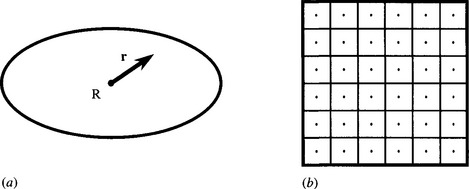
Figure 23.6 Object shape and method of sampling. (a) Object shape, showing reference point R and vector r pointing to a general location xR + r. (b) Image and sampling points, with associated tiling squares.
Unfortunately, it will not be possible to find a set of sampling point locations such that the “tiling” produced by the resulting maps of possible reference point positions covers the whole image without overlap. Thus, there will normally be some overlap (and thus loss of efficiency in locating objects) or some gaps (and thus loss of effectiveness in locating objects). The set of tiling squares shown in Fig. 23.6b will only be fully effective if square objects are to be located.
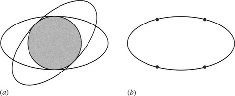
A more serious problem arises because objects may appear in any orientation. This prevents an ideal tiling from being found. It appears that the best that can be achieved is to search the image for a maximal rotationally invariant subset of the shape, which must be a circle, as indicated in Fig. 23.7a. Furthermore, as no perfect tiling for circles exists, the tiling that must be chosen is either a set of hexagons or, more practically, a set of squares. This means that the speedup factor for object location will be significantly less than n, though it will still be substantial.
23.4.2 Application to Grain Inspection
A prime application for this technique is that of fast location of grains on a conveyor in order to scrutinize them for damage, varietal purity, sprouting, molds, and the like. Under these circumstances, it is best to examine each grain in isolation; specifically, touching or overlapping grains would be more difficult to cope with. Thus, the grains would need to be spread out with at most 25 grains being visible in any 256 × 256 image. With so much free image space there would be an intensive search problem, with far more pixels having to be considered than would otherwise be the case. Hence, a very fast object location algorithm would be of special value.
Wheat grains are well approximated by ellipses in which the ratio of semimajor (a) to semiminor (b) axes is almost exactly two. The deviation is normally less than 20%, though there may also be quite large apparent differences between the intensity patterns for different grains. Hence, it was deemed useful to employ this model as an algorithm optimization target. First, the (nonideal) L × L square tiles would appear to have to fit inside the circular maximal rotationally invariant subset of the ellipse, so that ![]() i.e.,
i.e., ![]() This value should be compared with the larger value
This value should be compared with the larger value ![]() that could be used if the grains were constrained to lie parallel to the image x-axis—see Fig. 23.7b. (Here we are ignoring the dimensions
that could be used if the grains were constrained to lie parallel to the image x-axis—see Fig. 23.7b. (Here we are ignoring the dimensions ![]() for optimal rectangular sampling tiles.)
for optimal rectangular sampling tiles.)
Another consequence of the difference in the shape of the objects being detected (here ellipses) and the tile shape (square) is that the objects may be detected at several sample locations, thereby wasting computation (see Section 23.4.1). A further consequence is that we cannot merely count the samples if we wish to count the objects. Instead, we must relate the multiple object counts together and find the centers of the objects. This also applies if the main goal is to locate the objects for inspection and scrutiny. In the present case, the objects are convex, so we only have to look along the line joining any pair of sampling points to determine whether there is a break and thus whether they correspond to more than one object. We shall return later to the problem of systematic location of object centers.
For ellipses, it is relevant to know how many sample points could give positive indications for any one object. Now the maximum distance between one sampling point and another on an ellipse is 2a, and for the given eccentricity this is equal to 4b, which in turn is equal to ![]() Thus, an ellipse of this eccentricity could overlap three sample points along the x-axis direction if it were aligned along this direction. Alternatively, it could overlap just two sample points along the 45° direction if it were aligned along this direction, though it could in that case also overlap just one laterally placed sample point. In an intermediate direction (e.g., at an angle of around arctan 0.5 to the image x-axis), the ellipse could overlap up to five points. Similarly, it is easy to see that the minimum number of positive sample points per ellipse is two. The possible arrangements of positive sample points are presented in Fig. 23.8a.
Thus, an ellipse of this eccentricity could overlap three sample points along the x-axis direction if it were aligned along this direction. Alternatively, it could overlap just two sample points along the 45° direction if it were aligned along this direction, though it could in that case also overlap just one laterally placed sample point. In an intermediate direction (e.g., at an angle of around arctan 0.5 to the image x-axis), the ellipse could overlap up to five points. Similarly, it is easy to see that the minimum number of positive sample points per ellipse is two. The possible arrangements of positive sample points are presented in Fig. 23.8a.
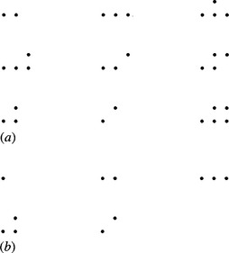
Fortunately, this approach to sampling is overrigorous. Specifically, we have insisted upon containing the sampling tile within the ideal (circular) maximal rotationally invariant subset of the shape. However, what is required is that the sampling tile must be of such a size that allowance is made for all possible orientations of the shape. In the present example, the limiting case that must be allowed for occurs when the ellipse is oriented parallel to the x-axis. It must be arranged that it can just pass through four sampling points at the corners of a square, so that on any infinitesimal displacement, at least one sampling point is contained within it. For this to be possible, it can be shown that ![]() , the same situation as already depicted in Fig. 23.7b. This leads to the possible arrangements of positive sampling points shown in Fig. 23.8b—a distinct reduction in the average number of positive sampling points, which leads to useful savings in computation. (The average number of positive sampling points per ellipse is reduced from ∼3 to ∼2.)
, the same situation as already depicted in Fig. 23.7b. This leads to the possible arrangements of positive sampling points shown in Fig. 23.8b—a distinct reduction in the average number of positive sampling points, which leads to useful savings in computation. (The average number of positive sampling points per ellipse is reduced from ∼3 to ∼2.)
Object location normally takes considerable computation because it involves an unconstrained search over the whole image space. In addition, there is normally (as in the ellipse location task) the problem that the orientation is unknown. This contrasts with the other crucial aspect of inspection, that of object scrutiny and measurement, in that relatively few pixels have to be examined in detail, requiring relatively little computation. The sampling approach we have outlined largely eliminates the search aspect of object location, since it quickly eliminates any large tracts of blank background. Nevertheless, the problem of refining the object location phase remains. One approach to this problem is to expand the positive samples into fuller regions of interest and then to perform a restricted search over these regions. For this purpose, we could use the same search tools that we might use over the whole image if sampling were not being performed. However, the preliminary sampling technique is so fast that this approach would not take full advantage of its speed. Instead, we could use the following procedure.
For each positive sample, draw a horizontal chord to the boundary of the object, and find the local boundary tangents. Then use the chord-tangent technique (join of tangent intersection to midpoint of chord: see Chapter 12) to determine one line on which the center of an ellipse must lie. Repeat this procedure for all the positive samples, and obtain all possible lines on which ellipse centers must lie. Finally, deduce the possible ellipse center locations, and check each of them in detail in case some correspond to false alarms arising from objects that are close together rather than from genuine self-consistent ellipses. Note that when there is a single positive sampling point, another positive sampling point has to be found (say, L/2 away from the first).
A significantly faster approach called the triple bisection algorithm has recently been developed (Davies, 1998b). Draw horizontal (or vertical) chords through adjacent vertically (or horizontally) separated pairs of positive samples, bisect them, join and extend the bisector lines, and finally find the midpoints of these bisectors (Fig. 23.9). (In cases where there is a single positive sampling point, another positive sampling point has to be found, say, L/2 away from the first.) The triple bisection algorithm has the additional advantage of not requiring estimates of tangent directions to be made at the ends of chords, which can prove inaccurate when objects are somewhat fuzzy, as in many grain images. The result of applying this technique to an image containing mostly well-separated grains is shown in Fig. 23.10. This illustrates that the whole procedure for locating grains by modeling them as ellipses and searching for them by sampling and chord bisection approaches is a viable one. In addition, the procedure is very rapid, as the number of pixels that are visited is a small proportion of the total number in each image.
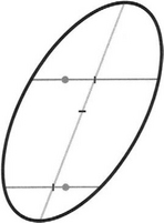
Figure 23.9 Illustration of triple bisection algorithm. The round spots are the sampling points, and the short bars are the midpoints of the three chords, the short horizontal bar being at the center of the ellipse.
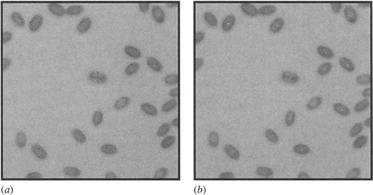
Figure 23.10 Image showing grain location using the sampling approach. (a) Sampling points. (b) Final center locations.
Finally, we show why the triple bisection algorithm is appropriate. First note that it is correct for a circle, for reasons of symmetry. Second, note that in orthographic projection, circles become ellipses, straight lines become straight lines, parallel lines become parallel lines, chords become chords, and midpoints become midpoints. Hence, choosing the correct orthogonal projection to transform the circle into a correctly oriented ellipse of appropriate eccentricity, we find that the midpoints and center location shown in the diagram of Fig. 23.9 must be validly marked. This proves the algorithm. (For a more rigorous algebraic proof, see Davies, 1999b.)
23.4.3 Summary
Motivated by the success of an earlier line-based sampling strategy (Davies, 1987l), Davies has shown that point samples lead to the minimum computational effort when the 180°-rotated object shapes form a perfect tiling of the image space. In practice, imperfect tilings have to be used, but these can be extremely efficient, especially when the image intensity patterns permit thresholding, the images are sparsely populated with objects, and the objects are convex in shape. An important feature of the approach is that detection speed is improved for larger objects, though naturally exact location involves some additional effort. In the case of ellipses, this process is considerably aided by the triple bisection algorithm.
The method has been applied successfully to the location of well-separated cereal grains, which can be modeled as ellipses with a 2:1 aspect ratio, ready for scrutiny to assess damage, varietal purity, or other relevant parameters.
23.5 Optimizing the Output for Sets of Directional Template Masks
Several earlier sections of this chapter highlighted the value of low-level operations based on template masks but did not enter into all the details of their design. In particular, they did not breach the problem of how to calculate the signal from a set of n masks of various orientations—a situation exemplified by the case of corner detection, for which eight masks are frequently used in a 3 × 3 window (see Section 23.2). The standard approach is to take the maximum of the n responses, though clearly this represents a lower bound on the signal magnitude l and gives only a crude indication of the orientation of the feature. Applying the geometry shown in Fig. 23.11, the true value has components:
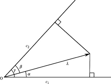
Finding the ratio between the components yields the first important result:
 (23.11)
and leads to a formula for tan a:
Next, we find from equation (23.9):
 (23.15)
On expansion we finally obtain the required symmetrical formula:
The closeness to the form of the cosine rule is striking and can be explained by simple geometry (Davies, 2000b).
Interestingly, equations (23.16) and (23.13) are generalizations of the standard vector results for edge detection:
which apply when γ = 90°. Specifically, the results apply for oblique axes where the relative orientation is γ.
23.5.1 Application of the Formulas
Before proceeding further, it will be convenient to define features that have 2π/m rotation invariance as m-vectors. It follows that edges are 1-vectors, and line segments (following the discussion in Section 23.2.1) are 2-vectors. In addition, it would appear that m-vectors with m > 2 rarely exist in practice.
So far we have established that the formulas given in Section 23.5 apply for 1-vectors such as edges. However, to apply the results to 2-vectors such as line segments, the 1:2 relation between the angles in real and quadrature manifolds has to be acknowledged. Thus, the proper formulas are obtained by replacing α, β, γ, respectively, by 2α, 2β, 2γ in the earlier equations. This leads to the components:
with 2γ = 90° replacing γ = 45° in the formula giving the final orientation:
as found in Section 23.2.1.
Finally, we apply these methods to obtain interpolation formulas for sets of 8 masks for both 1-vectors and 2-vectors. For 1-vectors (such as edges), 8-mask sets have γ = 45°, and equations (23.16) and (23.13) take the form:
For 2-vectors (such as line segments), 8-mask sets have γ = 22.5°, so 2γ = 45°, and the relevant equations are:
23.5.2 Discussion
This section has examined how the responses to directional template matching masks can be interpolated to give optimum signals. It has arrived at formulas that cover the cases of 1-vector and 2-vector features, typified, respectively, by edge and line segments. Although there are no likely instances of m-vectors with m >2, features can easily be tested for rotation invariance, and it turns out that corners and most other features should be classed as 1-vectors. An exception is a symmetrical S-shape, which should be classed as a 2-vector. Support for classifying corners as 1-vectors arises as they form a subset of the edges in an image. These considerations mean that the solutions arrived at for 1-vectors and 2-vectors will solve all the foreseeable problems of signal interpolation between responses for masks of different orientations. Thus, the main aim of this section is accomplished—to find a useful nonarbitrary solution to determining how to calculate combined responses for n-mask operators.
Oddly, these useful results do not seem to have been reported in the earlier literature of the subject.
23.6 Concluding Remarks
The topic of cereal grain inspection is ostensibly highly specialized. Not only is it just one aspect of automated visual inspection, but also it covers just one sector of food processing. Yet its study has taken these topics to the limits of the capabilities of a number of algorithms, and some very pertinent theory has been exercised and developed. This effort has made the chapter considerably more generic than might have been thought a priori. Indeed, this is a major reason for the rather strange inclusion of a section on template matching using sets of directional masks late on in the chapter. It was needed to advance the discussion of the subject, and if included in Part 1 of the book as a further aspect of low-level vision, it might have been regarded as a rather boring, unimportant addition. On the other hand, its presence in the present chapter emphasizes that not all the theory that needs to be known, and might have been expected to be known, is actually available in the literature—and there must surely be many further instances of this waiting to the revealed. In addition, there is a tendency for inspection and other algorithms to be developed ad hoc, whereas there is a need for solid theory to underpin this sort of work and, above all, to ensure that any techniques used are effective and robust. This is a lesson worth including in a volume such as the present one, for which practicalities and theory are intended to go hand in hand.
Food inspection is an important aspect of automated visual inspection. This chapter has shown how bulk cereals may be scrutinized for insects, rodent droppings, and other contaminants. The application is subject to highly challenging speed constraints, and special sampling techniques had to be developed to attain the ultimate speeds of object location.
23.7 Bibliographical and Historical Notes
Food inspection is beset with problems of variability; the expression “Like two peas” gives a totally erroneous indication of the situation. Davies has written much about this over the past many years, the position being summed up in his book and in more recent reviews (Davies, 2001a, 2003d). Graves and Batchelor (2003) have edited a volume that collects much further data on the position.
The work on insect detection described in this chapter concentrates on the linear feature detector approach, which was developed in a series of papers already cited, but founded on theory described in Davies (1997g, 1999f), and Davies et al. (2002, 2003a, 2003b). (For other relevant work on linear feature detection but not motivated by insect detection, see Chauduri et al., 1989; Spann et al., 1989; Koller et al., 1995; and Jang and Hong, 1998.) Zayas and Flinn (1998) offer an alternative strategy based on discriminant analysis, but their work targets the lesser grain borer beetle, which has a different shape, and the data and methods are not really comparable. That different methods are needed to detect different types and shapes of insects is obvious. Indeed, Davies’ own work shows that morphological methods are more useful for detecting large insects, as well as rodent droppings and ergot (Davies et al., 2003b; Ridgway et al., 2002). The issue is partly one of sensitivity of detection for the smaller insects versus functionality for the larger ones, coupled with speed of processing—optimization issues typical of those discussed in Chapter 29.
Recent work in this area also covers NIR (near infra-red) detection of insect larvae growing within wheat kernels (Davies et al., 2003c), although the methodology is totally different, being centered on the location of bright (at NIR wavelengths) patches on the surfaces of the grains.
The fast processing issue again arises with regard to the inspection of wheat grains, not least because the 30 tons of wheat that constitute a typical truckload contains some 6000 million grains, and the turnaround time for each lorry can be as little as three minutes. The theory for fast processing by image sampling and the subsequent rapid centering of elliptical shapes is developed in Davies (1997f, 1999b, 1999e, 2001b).
Sensitive feature matching is another aspect of the work described in this chapter. Relevant theory was developed by Davies (2000b), but there are other issues such as the “equal area rule” for designing template masks (Davies, 1999a) and the effect of foreground and background occlusion on feature matching (Davies, 1999c). These theories should all have been developed far earlier in the history of the subject and merely serve to show how little is still known about the basic design rules for image processing and analysis. A summary of much of this work appears in Davies (2000d).
1 A full derivation of this result appears in Section 8.6.1.
2 The proof of the concepts described here involves describing the signal in a circular path around the current position and modeling it as a sinusoidal variation, which is subsequently interrogated by two quadrature sinusoidal basis functions set at 0° and 45° in real space (but by definition at 90° in the quadrature space). The odd orientation mapping between orientation θ in the quadrature space and orientation ϕ in real space leads to the additional factor of one half in equation (23.3).
3 In the tests described in this section, all the images were processed with the same version of the algorithm; no thresholds were adjusted to optimize the results for any individual image.