In this chapter, you will examine the concept of a vector, a mathematical object describing relative positions in space. You already used vectors informally in the previous chapter, but now you will look at them in more detail. You will finish the chapter by looking at some calculations with matrices and how to use them to describe changes in space.
The first goal of this chapter is formally to describe vectors and see how to perform basic calculations with them.
A vector is like an instruction that tells you where to move. For example, imagine a pirate’s treasure map that says, “Take four steps north and three steps east; then dig.” These instructions describe a vector in two dimensions. First you go north. Then you go east. Or imagine being told in a hotel, “Go to the first floor, pass along the corridor, and then take the first door on the right.” These instructions describe a vector in three dimensions. You first go up. Then you go along the corridor. Then you turn right.
Vectors describe movement. With the pirate’s treasure map, it wouldn’t matter if you took one step west, four steps north, and then three steps east. You would still end up at the treasure—as long as you started in the right place. Vectors don’t have an intrinsic position in space. They simply tell you that if you start here, you will end up there.
Vectors are normally denoted by a letter in boldface, such as u or v. When working in Cartesian coordinates, you can indicate a vector by identifying the distances moved in the x-direction and the y-direction. This information is usually provided in a column array, which takes the form ![]() . For example, the vector illustrated in Figure 5.1 is communicated with
. For example, the vector illustrated in Figure 5.1 is communicated with ![]() . Because you are moving in a negative x-direction, the value in the x position of the vector is negative. These values are called the components of the vector in the x- and y-directions.
. Because you are moving in a negative x-direction, the value in the x position of the vector is negative. These values are called the components of the vector in the x- and y-directions.

Note
A vector is drawn as a straight line with an arrowhead indicating its direction. Although a duplicate is sometimes added in the middle of the line, the arrowhead is usually drawn at the end of the vector.
A vector can also be thought of as having two properties, a magnitude and a direction. The magnitude of a vector v, written |v|, is its length in space, which can be found from the Pythagorean Theorem. The magnitude of the vector ![]() is
is ![]() . In two dimensions, you can represent the direction by the angle the vector makes relative to an axis. A vector with magnitude 1 is called a unit vector. In two dimensions, it is equal to
. In two dimensions, you can represent the direction by the angle the vector makes relative to an axis. A vector with magnitude 1 is called a unit vector. In two dimensions, it is equal to ![]() for some angle α.
for some angle α.
Note
Some people prefer to write the magnitude of a vector without using boldface, so the magnitude of v would be written |v|. Since it can cause confusion, this convention is not observed in this book.
If you specify a starting point for a vector, it is called a position vector. An example of an instruction for a position vector is, “From the old oak tree, take three steps north.” Here, the old oak tree is the starting point. Mathematically, you usually choose a standard starting point, such as the origin in a Cartesian plane, and then measure all position vectors from this origin. As Figure 5.2 illustrates, if you draw a position vector on a graph starting from the origin, the coordinates of the end point are the same as the components of the vector. If you label the end points O and P, then you can write the vector as ![]() .
.
Subscripts are commonly employed to represent the components of a vector. As an example, the vector v might have the components (v1, v2). This is similar to the practice used in programming of identifying the components an array with indexes. In the syntax of a programing language, the components of an array v might be found by v[0], v[1], v[2], and so on. Note that the first item in an array is usually indexed as 0. In this book, the first item will be identified using v[1] rather than v[0].
Although there are two operations that resemble multiplication that you can perform on them, two vectors can’t be multiplied together in any simple way. You will see one approach in this chapter. Chapter 16 presents another. A third approach, used in programming, is pairwise multiplication. With this approach, the components are multiplied in pairs to create a new vector. While pairwise multiplication is not a standard mathematical tool, it will be explored in Chapter 19, where it is used on “vector-like” objects, such as colors.
In contrast to multiplication, addition of vectors is fairly straightforward. Likewise, you can easily multiply a vector by a scalar. Recall that a scalar value is a single value, in contrast to an array or vector.
To add two vectors together, add their components in pairs. Here is an example:
To multiply a vector by a scalar, multiply each component by the scalar. Here is an example:
As illustrated by the vectors on the left in Figure 5.3, multiplying a vector by a scalar changes its length proportionally but leaves the direction unchanged. The vector v, multiplied by 2, gives 2v. If the scalar is negative, however, the new vector faces in the opposite direction. Notice, that if v is multiplied by –1, then it becomes –v, and the result is a line with the arrowhead at the opposite end of the first.
In addition to reversing the arrowhead, you can designate a negative change in at least two other ways. For one, if the vector ![]() is v, then the negative of this vector is
is v, then the negative of this vector is ![]() . The order of the points is changed while the arrow continues to point in the same direction. Another approach is to use a negative sign—as has already been shown. The negative of vector v is expressed as –v.
. The order of the points is changed while the arrow continues to point in the same direction. Another approach is to use a negative sign—as has already been shown. The negative of vector v is expressed as –v.
For a non-zero vector v, if you divide it by its magnitude |v| or multiply it by the reciprocal of its magnitude ![]() , you get a unit vector. Unit vectors are sometimes indicated using the notation
, you get a unit vector. Unit vectors are sometimes indicated using the notation ![]() . A unit vector is called the normalized vector or norm of v.
. A unit vector is called the normalized vector or norm of v.
Figure 5.3 also illustrates the sum of two vectors. As is shown on the right side of Figure 5.3, the sum of two vectors is equal to the result of following one and then the other. (Recall that vectors don’t care what route you take to the end point; they only care about the final position.) In this instance, vector u takes a given direction. Then vector v takes another direction. The sum is the point reached by the two vectors.

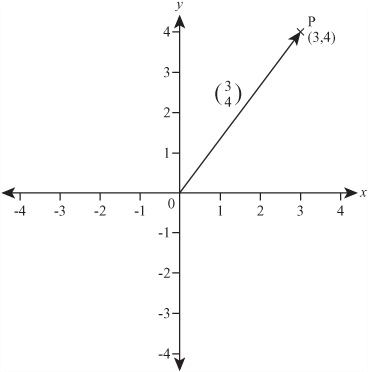
As is shown in Figure 5.4, the difference between two vectors is slightly more involved than addition of two vectors or multiplication of a vector by a scalar. If you consider two vectors, u and v, to be position vectors, one of the point P and the other of the point Q, so that ![]() , then the difference v – u is the vector
, then the difference v – u is the vector ![]() .
.
The reason this works is that if you start at P, follow the vector –u, and then the vector v, you end up at Q, so ![]() .
.
Such calculations are surprisingly powerful. As an example of what they can accomplish, consider the position vector of the mid-point of the line PQ in Figure 5.4. How is this found? If you start at O, travel to P, then move half-way along the vector PQ, you reach the mid-point M. The vector ![]() is equal to
is equal to ![]() , which is also the mean of the vectors u and v. Similarly, the position vector of the centrum of a triangle is the mean of the position vectors of its vertices.
, which is also the mean of the vectors u and v. Similarly, the position vector of the centrum of a triangle is the mean of the position vectors of its vertices.
Some programming languages have innate support for vector calculations. They allow you to add arrays and multiply them by scalars using precisely the rules described in the previous sections. 3-D engines usually include functions for calculating the magnitude and norm of a vector. To demonstrate how such functions are implemented, here is a set of functions for the calculations introduced so far.
The first function, addVectors(), adds two vectors, v1 and v2:
function addVectors(v1, v2)
   // assume vl and v2 are arrays of the same length
   set newVector to an empty array
   repeat for i=1 to the length of v1
      append v1[i]+v2[i] to newVector
   end repeat
   return newVector
end function
The scaleVector() function takes a vector v and scales it by a factor s:
function scaleVector(v, s)
   repeat for i=1 to the length of v
      multiply v[i] by s
   end repeat
   return v
end function
The magnitude() function provides the magnitude of a vector v:
function magnitude(v)
   set s to 0
   repeat with i=1 to the length of v
      add v[i]*v[i] to s
   end repeat
   return sqrt(s)
end function
The norm() function normalizes a vector:
function norm(v)
   set m to magnitude(v)
  // you can't normalize a zero vector
   if m=0 then return "error"
   return scaleVector(v,1/m)
end function
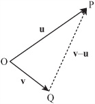
Consider one more important calculation, the angle between two vectors. You’ll see an easier way to calculate this later in the chapter, but for the moment, look back at Figure 5.4. Notice that the vectors u, v and u – v form a triangle OPQ. The result of this is that you can use the cosine rule to find any of the angles from the magnitude of these three vectors. In particular, you can find the angle θ between u and v using the following approach:
Here is a function that implements this equation:
function angleBetween(vector1, vector2)
   set vector3 to vector2-vector1
   set m1 to magnitude(vector1)
   set m2 to magnitude(vector2)
   set m3 to magnitude(vector3)
   // it makes no sense to find an angle with a zero vector
   if m1=0 or m2=0 then return "error"
   if m3=0 then return 0 // the vectors are equal
   return acos((m2*m2+m1*m1-m3*m3)/(2*m1*m2))
end function
If two vectors are perpendicular, they are also called normal. In two dimensions, it is simple to find the perpendicular to a given vector ![]() . To do so, invert the vector and take the negative of one component:
. To do so, invert the vector and take the negative of one component: ![]() . To see why this works, consider the vector as a position vector and remember your trick for fast rotation by 90°. Since any scalar multiple of this vector is still perpendicular to the original vector, it doesn’t matter which component you make negative. Multiplying by –1 gives you the same vector in the other direction. Here is a function that accomplishes this task:
. To see why this works, consider the vector as a position vector and remember your trick for fast rotation by 90°. Since any scalar multiple of this vector is still perpendicular to the original vector, it doesn’t matter which component you make negative. Multiplying by –1 gives you the same vector in the other direction. Here is a function that accomplishes this task:
function normalVector(vector)
   return vector(-vector[2],vector)
end function
Two vectors are perpendicular if and only if the sum of the products of their components is zero. With the normalVector() function, the product of the x-component of each vector is –ab and the product of the y-components is ab, so their sum is zero, as required. You’ll look at this further in a moment.
Many day-to-day quantities are best measured with vectors, and it is worth looking at them here since by doing so you gain a much clearer idea of what a vector is and why it is important. When applied to vectors, several terms used commonly in general contexts take on specific meanings. The following list provides a summary of a few of these terms.
Distance. This is a scalar quantity, and it measures the length of the shortest line between two points.
Displacement. If you identify two points connected by a vector, then the vector represents the displacement of the two points.
Speed. This is a scalar quantity. It measures the distance something travels in a certain time.
Velocity. A vector represents velocity, and velocity is the displacement in a given amount of time.
Mass. Mass is measured as a scalar. It is how much force is required to move something. The direction of the movement is irrelevant.
Weight. Weight is measured as a vector. It is the force required in a particular direction to keep something in the same place against the pull of gravity.
One common factor with these terms is that, informally, distance and displacement, speed and velocity, and mass and weight are often used interchangeably. For example, you describe an object as having a certain weight when, speaking precisely, you are describing its mass. Again, a train is described as traveling with a velocity of 100 km/hr when in fact this is its speed. Thinking in terms of vectors does not come naturally to most people.
However, in this context, it is important to distinguish between technical and non-technical usage. Later on, when you meet Newton’s Laws, you will talk about forces changing an object’s velocity. It is perfectly possible for an object to change velocity without changing speed. Think about a ball on the end of a string moving in a circle. Its direction of travel is changing constantly, but its speed is constant. Describing this in terms of vectors makes things simple. The velocity of an object is a vector, its speed is the magnitude of this vector. Thus, its velocity is changing, but its speed is not.
At this point, it is beneficial to spend a little time looking at how you can use vectors to perform calculations. Pay close attention to this section. In later chapters, you will be using these ideas extensively, particularly when dealing with collision detection and resolution.
Using vectors provides a convenient way to describe the relationship between points on a plane. For example, you have already encountered the word parallel. Two infinite lines are said to be parallel if either there is no point that lies on both lines, or if all points on one line are also on the other (in other words, if they are the same line). While this works well for infinite lines, it proves to be slightly more complicated for the kinds of lines you deal with most of the time, which have end points. Such lines are called line segments.
Using vectors, you can simplify the definition. Two lines are parallel if for any distinct points P and Q on one line, and P’ and Q’ on the other, there is some scalar a such that
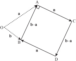
You can also use vectors to provide a recipe for creating shapes on the plane. For example, as is illustrated in Figure 5.5, given two points A and B with position vectors a and b, you can draw a square. You do so by first finding the normal of ![]() . This is also expressed as b – a. You call this vector n and assume that n has the same magnitude as b – a. (If this is not so, then you must scale it to the right length—a fairly easy task.) Now construct the points C and D using the calculations c = a + n and d = b + n. Notice that d – c = b – a and that
. This is also expressed as b – a. You call this vector n and assume that n has the same magnitude as b – a. (If this is not so, then you must scale it to the right length—a fairly easy task.) Now construct the points C and D using the calculations c = a + n and d = b + n. Notice that d – c = b – a and that ![]() is perpendicular to
is perpendicular to ![]() . Given these preliminaries, the points A, B, D, C form a square.
. Given these preliminaries, the points A, B, D, C form a square.
Note
With respect to Figure 5.5, notice that there are two possible squares that can be drawn on the line segment, depending on the direction chosen for the normal vector n.
Constructing an equilateral triangle is just as simple as constructing a square. You start with a little trigonometry. The length of the line from a vertex of an equilateral triangle to the mid-point of the opposite side is ![]() times the length of a side. (This is proved using the Pythagorean Theorem.) If you have two vertices, A and B, you can construct the third vertex C using
times the length of a side. (This is proved using the Pythagorean Theorem.) If you have two vertices, A and B, you can construct the third vertex C using ![]() . Here, n is the normal vector to b–a. Recall that
. Here, n is the normal vector to b–a. Recall that ![]() is the position vector of the mid-point of A and B.
is the position vector of the mid-point of A and B.
You can use similar constructions to create more complex shapes. At the end of this chapter, Exercise 5.1 challenges you to write a set of functions for creating shapes such as arrowheads and kites. The great advantage of such functions is that they can be easily parameterized to create a large number of variants on the same theme. As an example, here is a function that will create a whole family of letter As:
function createA(legLength, angleAtTop, serifProp, crossbarProp,
                    crossbarHeight, serifAlign, crossbarAlign)
   // serifProp, crossbarHeight, crossbarProp,
   // serifAlign and crossbarAlign should be values from 0 to 1
   // angleAtTop should be in radians
   set halfAngle to angleAtTop/2
   set leftLeg to legLength*array(-sin(halfAngle), cos(halfAngle))
   set rightLeg to array(-leftLeg, leftLeg[2])
   set crossbarStart to leftLeg*crossbarHeight
   set crossbarEnd to rightLeg*crossbarHeight
   set crossbar to crossbarProp*(crossbarEnd-crossbarStart)
   add crossbarAlign*(1-crossbarProp)*
                 (crossbarEnd-crossbarStart) to crossbarStart
   set serif to serifProp*(rightLeg-leftLeg)
   set serifOffset to serifAlign*serif
   set start to array(0,0)
   drawLine(start, leftLeg)
   drawLine(start, rightLeg)
   drawLine(crossbarStart, crossbarStart+crossbar)
   drawLine(leftLeg-serifOffset, leftLeg-serifOffset+serif)
   drawLine(rightLeg-serifOffset, rightLeg-serifOffset+serif)
end function
Figure 5.6 illustrates letters drawn using an implementation of this function. One of the most interesting side-effects of this approach is that you can take parameters of this kind and carry them across to related letters, creating a font in a similar style.

Note
With respect to Figure 5.6, if you find this kind of thing interesting, you might also want to look at Douglas Hofstadter’s Letter Spirit project, which explores the question of what it means for a font to be in a similar “style.”
The discussion of vectors thus far in this chapter has been building up to one of the most fundamental questions in programming, one that is especially important in game development. How do you move this from here to there? Consider Figure 5.7: the stick figure is moving from point P to point Q. Say that the stick figure’s game name is Jim, and its gender is male. If Jim is at (a, b) and walks to (c, d), what path does he follow?

To solve this problem, you can break it down into its constituent parts:
At time 0, Jim is at P = (a, b).
At time T, Jim is at Q = (c, d).
You want to know Jim’s coordinates at time t, where 0 <=t <= T
To proceed, it is necessary to introduce the concepts of speed and velocity. Start by looking at the problem in terms of vectors. In the time period of length T, Jim moves straight along the vector ![]() , which is
, which is ![]() . This is called his displacement z. The length of this vector,
. This is called his displacement z. The length of this vector, ![]() , is the distance Jim travels.
, is the distance Jim travels.
If you divide distance traveled by the time taken, you get the speed of the journey, measured as a unit of distance divided by a unit of time, such as a meter per second, or ms-1. The speed is the distance traveled in each time unit. Velocity is the displacement vector divided by the time taken, which is the vector traveled in each time unit. Given this work, you know that Jim’s velocity is ![]() .
.
Now you want to know where Jim is to be found at a time t. To discover this, consider that he has gone a proportion t/T of the way along the vector ![]() . Considering that t = mT, you say that this proportion is m, Jim’s position vector is given by
. Considering that t = mT, you say that this proportion is m, Jim’s position vector is given by
Note
Speed is a little more subtle than is presented in the previous discussion. If you travel in a long circle, ending up where you started, your displacement is zero, so your total velocity is also zero. Likewise, your mean velocity is zero. However, your mean speed is not zero. Instead, it is equal to the circumference of the circle (the distance traveled) divided by the time taken. Speed is found using the length of the path traveled, not the length of the eventual vector. When moving in a straight line, however, this is immaterial.
When programming motion, it is often useful to pre-calculate values. In object-oriented programming, you usually represent a sprite on the screen with a specific object. You usually send this object from one location to another by a method that takes the new location and time as a parameter. If you develop a function to accomplish this task, it is likely to take the form of the calculateTrajectory() function:
function calculateTrajectory(oldLocation, newLocation, travelTime)
   if time=0 then
      justGoThere(newLocation)
   otherwise
      set displacement to newLocation-oldLocation
      set velocity to displacement/travelTime
      set startTime to the current time
      set stopPosition to newLocation
      set startPosition to oldLocation
   end if
end function
Having calculated the trajectory, whenever you want to update the position of the sprite, you can calculate the new position directly. The currentPostion() function accomplishes this task:
function currentPosition()
   set time to the current time-startTime
   if time>travelTime then
      set current position to stopPosition
   otherwise
      set current position to startPosition+velocity*time
   end if
end function
Note
The currentPostion() function method uses one variable you can manage without—startPosition(). Can you think of how you could do the same thing without remembering your starting position? As a hint, try counting down instead of up.
Generally, the best approach to constructing functions for determining the current position of an object is to give your object a standard speed and calculate the time to travel from there. This approach is addressed in Exercise 5.2 at the end of this chapter.
Vector motion is not useful only for straight lines. You have already seen how simple shapes can be described by a sequence of vectors. In this section, you see this activity extended to encompass curved motion created when the velocity of a particle changes as the particle moves.
Note
The word particle is mathematical shorthand for something that is moving in an indeterminate way. Particles are supposed to be infinitely small, although they can have properties like electrical charge or mass, depending on the circumstances. Since it is not a word that has an alternative meaning in programming, you frequently use the term particle to describe a moving element (a sprite) on the screen.
Consider Jim encountering a different scenario of motion, as illustrated in Figure 5.8. As shown on the left side of Figure 5.8, instead of approaching point Q directly, in this instance, Jim wants to skirt around it. He can do this by adding a multiple of the normal vector to his trajectory. Given this approach, Jim does not move directly along the line PQ; instead, he travels a short distance along it and a short distance perpendicular to it, to the point P’. Then, with the next step, he does the same thing, moving a little perpendicular to P’Q to P″, and so on.
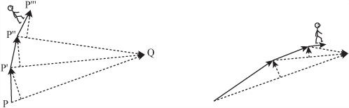
If you extend this scenario far enough, you can see that the path Jim follows can be a spiral. This becomes apparent in the path represented on the right side of Figure 5.8. Here, the tightness of the spiral depends on how large the normal vector is when compared to the inward speed. If the tangential component is zero, then Jim travels along a straight line. If it is greater than zero but small, he travels along a slightly curved path. If it is large, he spirals in gradually. If it is infinite, on the other hand, he simply moves in a circle around Q.
Generally speaking, because the time steps of a particle moving on a screen are not infinitely small, the path that the particle travels will not be mathematically accurate. Still, the behavior will resemble what has been described with respect to Jim. The curvedPath() function moves a particle in a curved path of this kind:
function curvedPath(endPoint, currentPoint,
                    speed, normalProportion, timeStep)
   set radius to endPoint-currentPoint
   if magnitude(radius)<speed*timeStep then
      set current position to endPoint
   otherwise
      set radialComponent to norm(radius)
      set tangentialComponent to
          normalVector(radialComponent)*normalProportion
      set velocity to speed*norm(radialComponent+tangentialComponent)
      set current position to currentPoint+velocity
   end if
end function
You can do some wacky things if you remove vectors from real life and imagine them as things in their own right. For example, with reference to the curvedPath() function presented in the previous section, the value of normalProportion is equivalent to a unit length vector ![]() , where α is equal to
, where α is equal to atan(normalProportion). What happens if you let this vector vary? For example, consider what happens if you give the vector its own “velocity” by varying α at a constant speed around the circle. As illustrated by Figure 5.9, if you do this, some fantastic paths result.

Creating a function that generates such paths involves altering the approach used in the previous example. The madPath() function shows one approach:
function madPath(endPoint, currentPoint,
                 currentAlpha, speed, alphaSpeed, timeStep)
   set radius to endPoint-currentPoint
   if magnitude(radius)<speed*timeStep then
      set current position to endPoint
   otherwise
      set radialComponent to norm(radius)
      set newAlpha to currentAlpha+alphaSpeed*timeStep
      set tangentialComponent to
                      normalVector(radialComponent)*tan(newAlpha)
      set velocity to speed*norm(radialComponent+tangentialComponent)
      set current position to currentPoint+velocity
   end if
end function
Thinking of an abstract quantity in terms of vectors provides you with a powerful tool. As powerful a tool as it is, however, it is often difficult to use it to arrive at the results you want. For now, remember the idea of varying the velocity vector over time. This leads to the idea of acceleration.
In this section, you examine techniques for creating and solving vector equations.
Any two non-parallel vectors that share a single defined origin can be used to describe any point on a plane. If u and v are non-parallel vectors, then any vector on the plane can be described uniquely in the form au + bv, where a and b are scalars. When you employ this approach to manipulating, you use u and v as a basis. One example of this involves the vectors ![]() , often denoted i and j. Since the vector
, often denoted i and j. Since the vector ![]() is equal to ai + bj, the components of the vector translate directly into the basis description. Because the basis vectors are orthogonal (perpendicular to each other) and normalized (of unit length), their relationship to each other is described as an orthonormal basis.
is equal to ai + bj, the components of the vector translate directly into the basis description. Because the basis vectors are orthogonal (perpendicular to each other) and normalized (of unit length), their relationship to each other is described as an orthonormal basis.
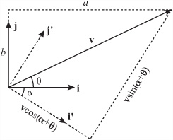
Sometimes it is useful to use a different basis. For example, as illustrated by Figure 5.10, it is often practical to think in terms of the radial and tangential components of a motion, which is the same as describing the velocity vector in terms of a new orthonormal basis directed toward the goal.
The advantage of doing this is that often the components in these two directions can be considered independently. As is described in later chapters, when a force is directed along one vector, the velocity perpendicular to that vector is unchanged.
Note
The word component has a dual meaning. With a given orthonormal, if you have v = pa + qb, then you can use the expression “component of v in the a-direction” to designate either the vector pa or just the number p. It is usually clear from context which of these is intended. When programming, you can define two functions, component(vector1, vector2) and componentVector(vector1, vector2), to distinguish between them.
In Figure 5.10, the vector v is to be converted from the basis i, j to the basis i’, j. The angle between i and i’ is α and the angle between v and i is θ. You have drawn a rectangle around the vector parallel to the new axes, and you can see that the magnitude of the component in the direction i’ is equal to |v|cos(θ–α). In the direction j’, the magnitude is equal to |v|sin(θ–α). Further, you can calculate the angles θ and α directly from the components of v and i’ in the directions of i and j. For example, if v is the vector ![]() =ai + bj then θ =
=ai + bj then θ = atan(b, a).
To summarize this discuss in terms of a function, the switchBasis() function takes two arguments, the vectors v and k, and returns four values. The four values are the orthonormal vectors i’ and j’ (where i’ is the normalized version of k) and the components a and b of v in the directions of i’ and j’. At the end, then, you know that v = ai’ + bj’.
function switchBasis(vector, directionVector)
   set basis1 to norm(directionVector)
   set basis2 to normal(basis1)
   set alpha to atan(basis1[2],basis1[1])
   set theta to atan(vector[2],vector[1])
   set mag to magnitude(vector)
   set a to mag*cos(theta-alpha)
   set b to mag*sin(theta-alpha)
   return new array(basis1, basis2, a, b)
end
Note
Notice that you have used the two-argument version of the atan() function introduced in Chapter 4.
You can also write two simpler functions that find a single component in a new basis. The first is the component() function:
function component(vector, directionVector)
   set alpha to atan(directionVector [2], directionVector [1])
   set theta to atan(vector[2],vector[1])
   set mag to magnitude(vector)
   set a to mag*cos(theta-alpha)
   return a
 end function
The second is the componentVector() function:
function componentVector(vector, directionVector)
   set v to norm(directionVector)
   return component(vector, directionVector)*v
end function
As becomes evident after a little study, the componentVector() and component() functions are likely to be more useful than the switchBasis() function.
Although the methods you’ve seen so far in this chapter for finding angles and components of vectors are fairly simple, there is another way that is much more versatile. As you saw earlier, there is no natural way to multiply two vectors. However, one common operation you can perform involves the scalar product. As its name suggests, the scalar product is a function that combines two vectors to get a scalar answer.
The scalar product of the vectors u and v is written using a dot: u . v. Use of the dot is why the scalar product has become commonly known as the dot product. To calculate the scalar product, you take the sum of the products of the corresponding vector components. Here is an example:
What is the use of this type of operation? One approach to answering such a question is to consider what happens with the dot product of a given vector and the basis vector i. A basis vector is expressed as ![]() . This basis vector identifies the x-component of the vector. The dot product of this vector with a given vector j gives the y-component. Similarly, when you take the dot product of vector v with any unit vector u, you end up with the component of v in the direction of u.
. This basis vector identifies the x-component of the vector. The dot product of this vector with a given vector j gives the y-component. Similarly, when you take the dot product of vector v with any unit vector u, you end up with the component of v in the direction of u.
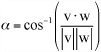
The dot product of two vectors v and w is equal to |v|×|w|× cos α where α is the angle between the two vectors. This means that you can use the dot product for a number of useful calculations. For example, the dot product of a vector with itself is the square of its magnitude. (This follows from the Pythagorean Theorem.) Also, you can find the angle between two vectors by using this approach:
The dot product has the following properties:
It is commutative:

It is distributive over addition:

Multiplying by a scalar gives

If two vectors are perpendicular then their dot product is zero, and vice versa.
As with regular numbers, you can do algebra with vectors. In fact, when working with simultaneous equations in Chapter 3, you have already done so in a disguised way. A vector equation might be something like this:
Any of the variables in this equation might be unknowns—the scalars a and b, or the vectors u, v, and w. However, with such equations, the most common situation is one in which you know the values of vectors but not the values of the scalars.
As illustrated by Figure 5.11, consider a problem in which you are trying to find the intersection point of the two lines AB and CD. You know the position vectors a, b, c, d of the four points A, B, C, D, and you are looking for the position vector of the point P, where the two lines cross.
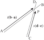
The trick here is to try to parameterize P. In other words, you must find a way to describe P in terms of the points A, B, C, D. All you know about P is that it lies on lines AB and CD. So what can you say about a point that lies on a particular line AB? To get to such a point, you can start at the origin O, travel to A, and then travel some distance along the vector AB. Since you don’t know how far you travel, you say it’s some value t. Therefore, to express the problem, you write
What is more, because P also lies on CD, you can say that
for some scalar s.
This gives you an equation for s and t:
Now this appears to be a single equation in two variables. However, it is really two equations in disguise, because it must be true separately for both the x- and y-coordinates of the basis. This means that you can separate the vector equation into two simultaneous linear equations:
where a1, b1, c1, d1 are the x-components of the vectors a, b, c, d. In other words, they are the x-coordinates of the points A, B, C, D. This is similar for a2, b2, c2, d2.
Note
It can be confusing to keep these various concepts distinct. For this reason, it is advisable to maintain a clear separation between the points, vectors, and components in a problem. Establishing this practice early on helps you when the problems get more complicated.
While simultaneous equations can be solved by the same methods you used previously—assigning values to t and s—you really need only one of the values to solve the problem. You’ve already gone through the process of solving simultaneous equations, so there is no need to retread that ground here. The intersectionPoint() function uses a simplified approach to the problem to take four vectors as arguments and return the intersection of the lines between them.
function intersectionPoint(a, b, c, d)
   set tc1 to b[1]-a[1]
   set tc2 to b[2]-a[2]
   set sc1 to c[1]-d[1]
   set sc2 to c[2]-s[2]
   set con1 to c[1]-a[1]
   set con2 to c[2]-a[2]
   set det to (tc2*sc1-tc1*sc2)
   if det=0 then return "no unique solution"
   set con to tc2*con1-tc1*con2
   set s to con/det
   return c+s*(d-c)
end function
Note
In the intersectionPoint() function, you might be wondering why the variable name det is used for the value (tc2*sc1-tc1*sc2). It stands for determinant, a term explained shortly.
You can also do the same thing in a different way starting with the position vectors of A and C and the vectors ![]() and
and ![]() :
:
function intersectionTime(p1, v1, p2, v2)
   set tc1 to v1[1]
   set tc2 to v1[2]
   set sc1 to v2[1]
   set sc2 to v2[2]
   set conl to p2[1]-p1[1]
   set con2 to p2[2]-p1[2]
   set det to (tc2*sc1-tc1*sc2)
   if det=0 then return "no unique solution"
   set con to sc1*con2-sc2*con1
   set t to con/det
   return t
end function
With the intersectionTime() function, instead of returning the point of intersection, the function returns the value of t. There is a good reason for this. As is illustrated by Figure 5.12, the values t and s are useful for more than determining the position of P. They also tell you the relationship of P to the points A, B, C, D. Suppose, for example, the value of t turns out to be 0.5. This means that P is equal to a + 0.5 (b – a), which is half-way along the line AB.
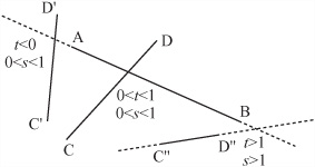
In general, if t is between 0 and 1, then P lies between the points A and B (with a value of 0 representing the point A, and 1 representing B). If t is greater than 1, then P lies somewhere beyond the point B. And if t is less than 0, then P lies behind the point A.
Similarly, s determines how far along the line, CD, P lies. If both s and t are in [0,1] point P actually lies on the intersection of the line segments AB and CD. In any other case, P lies on the projection of the lines to infinity.
In addition to the intersectionPoint() and intersectionTime() functions, you can create a slightly different function, one that finds the point where two line segments intersect. In addition to returning the value of t, this function is useful when working on collision detection.
function intersection(a, b, c, d)
   set tc1 to b[1]-a[1]
   set tc2 to b[2]-a[2]
   set sc1 to c[1]-d[1]
   set sc2 to c[2]-s[2]
   set con1 to c[1]-a[1]
   set con2 to c[2]-a[2]
   set det to (tc2*sc1-tc1*sc2)
   if det=0 then return "no unique solution"
   set con to tc2*con1-tc1*con2
   set s to con/det
   if s<0 or s>1 then return false
   if tc1<>0 then set t to (con1-s*sc1)/tc1
   otherwise set t to (con2-s*sc2)/tc2
   if t<0 or t>1 then return "none"
   return t
end function
In the functions given in the three previous sections, situations might arise in which the value det is zero. In this case the lines AB and CD are parallel. If this happens, at least two possibilities arise:
If the segments AB and CD lie along the same line (the points A, B, C, D are collinear), then either they intersect for some continuous stretch, or they are separate.
If they don’t lie on the same line, then they do not intersect at all.
Distinguishing these three possibilities isn’t particularly difficult. To do so, you use another vector equation. If A, B, C, D are collinear then any one of the points can be described in terms of the other two. For example, c = a + k (b – a) for some k. And, if the value of k in this equation is between 0 and 1 then C lies somewhere between A and B, with the same holding true for the equivalent parameter 1 and the point D. As long as either C or D lies within the segment AB, the lines intersect.
A matrix, like a vector, is a mathematical array representing tabular information. The plural of matrix is matrices. This section briefly discusses matrices and the basics of matrix arithmetic.
To understand the difference between a matrix and a vector, consider first that a vector is a one-dimensional array. It is a list of components representing motion in a fixed number of directions. Even a vector in three dimensions, such as the vector ![]() , is still a one dimensional object. It has one value for each of the three directions.
, is still a one dimensional object. It has one value for each of the three directions.
In contrast, a matrix has values in two directions. To represent values, the values of a matrix are represented like a table enclosed in brackets: ![]() . The horizontally aligned values are rows. The vertically aligned values are columns. You can think of a matrix, then, as a table of values relating rows to columns. For example, here is a table of prices of electrical goods:
. The horizontally aligned values are rows. The vertically aligned values are columns. You can think of a matrix, then, as a table of values relating rows to columns. For example, here is a table of prices of electrical goods:

Looking along the Gizmo row and locating the price under the Large column, you can determine the price of a large gizmo—$20.00.
Representing matrices as rows and columns allows you to define them, but if you then want to use matrices as parts of equations, an abbreviated form is needed. Accordingly, matrices are usually represented by small or capital letters in boldface (G, for example). To show that a given letter designates a given matrix, you assign the matrix to the letter, as follows:

To relate the rows and columns of a matrix, a times sign (×) is used. Thus, because it has three rows and three columns, G is a 3 × 3 matrix. With four columns, G would be a 3 × 4 matrix. If it has the same number of rows as columns, a matrix is said to be square. While you’re reviewing definitions, you can also define the transpose of a matrix. Represented with a superscript T, a transpose matrix is a matrix with the rows and columns exchanged. Here is a transpose of matrix G.
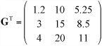
The transpose of an n × m matrix is m × n in size. Notice that taking the transpose leaves the numbers on the diagonal extending from the left at the top to the bottom on the right unchanged. This is called the leading diagonal of the matrix.
Since a vector can be represented as a n × 1 matrix, you can use the transpose notation to represent it in row form. In this case, then, the n × 1 matrix becomes a 1 × n matrix. As a result, instead of writing ![]() , you may write (1 2 3)T. In addition to using rounded braces to identify matrices, angled brackets are also commonly employed. Using this convention, a row vector is shown as
, you may write (1 2 3)T. In addition to using rounded braces to identify matrices, angled brackets are also commonly employed. Using this convention, a row vector is shown as ![]() .
.
In programming, a matrix must be represented as an array of arrays. Consider how to represent a 3 × 3 matrix. One array represents the rows. Within this array, there are three more arrays. Each of the arrays must have three elements, each of which represents a value in a column. So the matrix G would be the array [[1.2, 10, 5.25],[3, 15, 8.4], [4.5, 20, 11]].
The notion of a determinant was introduced previously in this chapter. A square matrix has an associated value called the determinant of the matrix. Somewhat equivalent to the length of a vector, the determinant is a fundamental feature of the matrix. To denote the determinant, vertical bars are used. The determinant of M is written |M|. If this were a function, you could express it as det(M).
The determinant of a matrix is the same as the determinant of its transpose. For a 2 × 2 matrix ![]() , the determinant is equal to ad – bc. For larger matrices, the formula is more complicated, although you can write it reasonably simply using a recursive function that takes a square matrix M as an argument. The
, the determinant is equal to ad – bc. For larger matrices, the formula is more complicated, although you can write it reasonably simply using a recursive function that takes a square matrix M as an argument. The determinant() function provides one approach to this technique:
function determinant(m)
   set size to the number of elements in m
   if size=1 then return m[1][1]
   set mult to 1
   set sum to 0
   repeat for i =1 to size
      set el to m[1][i]
      set newmatrix to an empty array
      repeat for j=2 to size
         append m[j] to newmatrix
         remove the i’th element of this row
      end repeat
      add el*mult*determinant(newmatrix) to sum
      multiply mult by -1
   end repeat
   return sum
end function
Note
Matrices, vectors and scalars are all special cases of a general class of mathematical arrays called tensors, which are ways to describe a variation in values over regions of mathematical space. Working with tensors tends to be more an exercise in number-juggling than anything else. Tensors are an essential part of any physics of fields, such as general relativity or electromagnetism. They also turn up in rotational physics, where you encounter the phrase “inertia tensor.”
Matrix arithmetic, like vector arithmetic, usually begins with operations involving scalars and matrices. It progresses from there to operations involving matrices and matrices. To multiply a matrix by a scalar, you multiply each element within the matrix by the scalar:
To explore the simplest of operations involving two matrices, you can add two matrices of the same size by simply adding their equivalent elements:
Such operations are easy to follow, but the situation changes when matrices are multiplied by matrices. Even then, however, the process is not overwhelming if expressed in simple terms. Consider, for example, multiply an l × n matrix L by an n × m matrix M.
To accomplish this, take the first element in the first row of L and multiply it by the first element in the first column of M. Do the same for each element of the first row and column of the matrices. Put the sum of these values in the top-left column of a new matrix N.
Continue this process for each pair of a row i of L and column j of M to get a value for the i’th row and j’th column of N. This will eventually give you an l × m matrix. Notice that this is only possible if the number of columns of L is the same as the number of rows of M.
The matrixMultiply() function takes two arguments, l and m, which are matrices to be multiplied. It then returns a matrix contained by the multiplied values of the two matrices.
function matrixMultiply(l, m)
   set n to a blank array
   repeat with i=1 to the number of rows of l
      set r to a blank array
      repeat with j=1 to the number of columns of m
         set sum to 0
         repeat with k=1 to the number of columns of l
            add l[i][k]*m[j][k] to sum
         end repeat
         append sum to r
      end repeat
      append r to n
   end repeat
   return n
end function
As becomes evident if you try it, multiplication of matrices is not commutative. In other words, LM ≠ ML. In fact, in general it is not even meaningful to multiply matrices in the reverse order. Even for square matrices, the result of multiplying is, as a rule, different depending on the order. On the other hand, the situation differs with transposes. You can say, for example, that if LM = N, then MTLT = NT.
Note
Notice that the product uTv, where u and v are column vectors, gives the dot product of u and v (or rather, a 1×1 matrix whose sole element is the dot product).
Although matrix multiplication is not commutative, it is associative: L (MN) = (LM)N. It is also distributive over addition: L (M+N) = LM+LN. For square matrices, matrix multiplication also preserves the determinant: |LM| = |L||M|.
For each size of square, there is a special identity matrix I, which leaves other matrices unchanged under multiplication: IM = MI = M. To apply this rule, it is necessary to select an identity matrix of the appropriate size for each multiplication. In each of the positions on the leading diagonal, the identity matrix has the value 1. Elsewhere, the value is 0. For example, the 2 × 2 identity matrix is ![]() .
.
For any square matrix M whose determinant is not zero, there is a unique inverse matrix M-1 such that MM-1 = M-1M = I. For a 2 × 2 matrix ![]() , the inverse is equal to
, the inverse is equal to ![]() . This gives you yet another way to solve simultaneous equations. You start by encoding a set of simultaneous equations as a matrix. Suppose the equations are as follows:
. This gives you yet another way to solve simultaneous equations. You start by encoding a set of simultaneous equations as a matrix. Suppose the equations are as follows:
This is equivalent to
where the vector (x y)T is a single unknown with two dimensions.
Now you left-multiply both sides of the equation by the inverse of the matrix:

Note
Note the use of the expression left-multiply. Because matrix multiplication is non-commutative, multiplying on the left or on the right are different operations.
So you now have a single matrix calculation to find the values of x and y, giving you the following:
As it happens, you can use a process similar to the one you used to solve simultaneous equations to find the inverse of matrices larger than 2 × 2. You perform linear operations (multiplying by a scalar and adding linear combinations) on the rows of the matrix in order to turn it into an identity matrix. If you perform the same operations on an original identity matrix, it turns into the inverse of your original matrix.
Like a vector, a matrix is best thought of as an instruction. A vector is an instruction to move in a certain direction. If you multiply a matrix and a vector together, you get a new vector, so a matrix is an instruction for how to interpret the vector. In fact, a matrix is a transformation of space. Here are some examples of matrix transformations in two dimensions:
If you take the matrix
 = nI and multiply it by any vector (v), you get the same vector multiplied by n. Since (nI)v = n (Iv) = nv this is not surprising. This vector represents a scale transformation, and any matrix with a determinant other than 1 (or zero) includes some element of scaling.
If you left-multiply the matrix
 by any vector, you get the vector with its x-coordinate reversed. In other words, the vector is reflected in the y-axis. Any matrix with a negative determinant is a reflection of some kind—as well as a possible scale.
If you left-multiply the matrix
 by any vector, you get the vector with its x- and y-coordinates switched. In addition, the x-coordinate is reversed, resulting in a normal vector, one rotated clockwise by 90° about the origin.
If you multiply the matrix
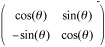 by any vector, you get the vector rotated clockwise by θ about the origin. Notice that because cos2(θ)+sin2(θ)=1, the determinant of this matrix is 1, so the vector is not scaled or reflected.
If you multiply the matrix
 by any vector, you get the vector skewed parallel to the x-axis by an amount proportional to the y component. This matrix represents a shear and has a determinant of 1.
Not all transformations can be represented by a matrix in this way. In particular, translations are achieved by adding a constant vector, rather than by a matrix multiplication. Every transformation centered on the origin can be represented by a matrix, and you can use matrix multiplication rules to calculate the combined results of several such transformations. For example, consider what you must do if you want to rotate a triangle by 75° clockwise about the origin, scale it to twice its size, and reflect it in the x-axis. One way to accomplish this is involves the following steps:
Multiply the position vector of each vertex of the triangle by the matrix
 to perform the rotation.
Multiply the resultant vector by the matrix
 .
.Multiply the resultant vector by the matrix
 .
.
This means that the end position of the vertex with position vector a is T(S(Ra))=(TSR)a. To transform it in one pass, if you start by calculating the matrix TSR, you can apply this matrix to all the vertices of the triangle and any others you happen to need.
As before, remember that matrix multiplication, and thus transformation, is not commutative. If you perform the three operations in a different order, you will get a different end result. To see how this makes sense, imagine turning left and then looking in a mirror. You get a different end result than when looking in the mirror and then turning the mirror image left.
Before finishing this topic, quickly have a look at what happens to the basis vectors ![]() under the transformation M =
under the transformation M = ![]() . You can see that you have
. You can see that you have ![]() . The columns of the matrix M give the results of transforming the basis vectors. This results in a couple of outcomes. First, if you know the result of a transformation on the basis vectors, you know everything there is to know about it. Second, you can use this result to calculate the transformation matrix.
. The columns of the matrix M give the results of transforming the basis vectors. This results in a couple of outcomes. First, if you know the result of a transformation on the basis vectors, you know everything there is to know about it. Second, you can use this result to calculate the transformation matrix.
One final useful property of a matrix is its set of eigenvectors and associated eigenvalues. These are a very handy way to characterize a matrix. In essence, an eigenvector is a vector that maps to a multiple of itself under a particular transformation. The multiple is called the eigenvalue for that vector. If p is an eigenvector of M, and λ is the corresponding eigenvalue, you have
Note
Strictly speaking, you should distinguish between right-eigenvectors and left-eigenvectors. While left-eigenvectors are similar to the eigenvector just explained, they are multiplied on the left of the matrix. Multiplied on the right of the matrix, right-eigenvectors are more common, and unless stated otherwise, when people talk about an eigenvector, they are talking about a right-eigenvector. As it is, however, even if the eigenvectors on left and right are different, the set of eigenvalues on each side is the same for any given matrix.
Write a set of functions such as drawArrowhead(linesegment, size, angle) and drawKite(linesegment, height, width), which create complex shapes from simple initial parameters.
Don’t just stick to these two shapes. Try making as many as you can think of. Try drawing letterforms as shown in the chapter. You might create variable fonts based on parameters of widths, heights, and angles. You might also create a simple 3-D effect that results in a “bevel” for a set of points.
Working from the example given in this chapter, write a function named calculateTrajectory(oldPosition, newPosition, speed), which pre-calculates the velocity vector and other necessary parameters of a movement.
The function should end up with the same set of parameters given by the calculateTrajectory () in this chapter.
In this chapter, you have covered the essentials of vector and matrix arithmetic and algebra, reviewing a few basic tools for thinking about space. You’ve seen how you can use vectors to describe positions and movement, and how to use them to perform complicated calculations like finding intersections of lines. In addition, you’ve also seen how matrices can be used to transform space and looked at the concept of a basis.
In the final chapter of Part I, you’ll return to algebra and, with the help of the topics presented in this and previous chapters, look at further ways to analyze functions.
What a vector is, how to describe it in terms of its components, and how to perform basic arithmetic such as adding, subtracting and scaling vectors
The meanings of the terms magnitude, norm and normal, and how to calculate them for a given vector
How to calculate the scalar (dot) product of two vectors, and what this operation means
How to use combinations of known vectors to describe a known position in space
How to parameterize a vector description to communicate a concept such as “a vector on the line AB”
How to find the components of a vector in a different direction (putting it into a different basis) both geometrically and by using the dot product
How to solve vector equations using linear simultaneous equation techniques, and how to use this to find intersections between lines
What a matrix is and how to perform matrix calculations
How to solve simultaneous linear equations with matrices
How to use matrices to create multiple transformations of space