When atoms gain and then lose energy, they emit the energy in the form of a wave of oscillating electric and magnetic fields. These fields are referred to collectively as electromagnetism. Depending on the amount of energy, electromagnetism has varying frequencies and wavelengths. Human bodies include detectors that respond to a certain ranges of these frequencies. In the form perceived by humans, this is called light. In precise terms, it is called visible light.

In the human eye, detectors of light are called rods and cones. These have different functions. The rod is sensitive to levels of brightness, and levels of brightness are created by differing wave amplitudes. Cones are sensitive to the frequency, and for this reason, they are a bit more complicated than rods. To start with, humans have three different kinds of cone, and each type of cone is sensitive to a different range of light. While one range is described as red, the other two are described as green and blue.

The fact that humans have three types of cones distinguishes them from other animals. Most mammals have two kinds of cone, limiting the colors that they see. At the same time, differences of cones do not mean only that limitations occur. Some animals can see ranges of light that humans consider invisible. Bees see ultra-violet light, and ultra-violate light has a higher frequency light than humans can see. Although not visually, snakes can detect light in the infra-red region, and infra-red light is of a lower frequency, again not naturally visible to humans.

Even though humans have cones that detect red, green, and blue, it remains that they are able to see far more than only three colors. Since most light contains several overlapping waves with a broad range of frequencies, all three kinds of cone are activated to different levels, as are the rods, and this mixture of frequencies is discriminated (or experienced) as a single color. Even a single-wavelength beam that doesn’t precisely trigger one cone can be discriminated by the amount to which it activates the neighboring cones.

Colors emerge from differences of discrimination. Wavelengths halfway between pure red and pure green are experienced as yellow. Wavelengths halfway between green and blue are experienced as a sky-blue color called cyan. A mixture of blue and red is experienced as a purplish color called magenta. Generally, your visual system processes colors in a cycle characterized by red-yellow-green-cyan-blue-magenta-red. This cycle itself is a product of biological evolution and bears no direct relationship to the underlying wavelengths of light. Along the same lines, a mixture of lots of different wavelengths is experienced as white, while no light at all is experienced as black.

Computer engineers take advantage of the peculiarities of your visual system by mimicking them in the way computer monitors display colors. Each pixel of the monitor screen is made up of three separate emitters of red, green, and blue (RGB). Each emitter can take any value between off and on. For a high-resolution display, each can have a value between 0 and 255. When all three emitters are fully lit, a white dot is created. When none of the emitters is lit, a black dot appears. Depending on the power of your computer and the resolution of your monitor, you can create many different colors this way. In fact, on a truecolor scale, you can create 16,777,216 different colors. The truecolor scale is a convention sustained by the electronics industry and designates colors that can be defined using 256 shades of red, green, and blue.

In the context of linear algebra, you can represent each color by a 3-D RGB vector. The vector defines the size of each color by a real number between 0 and 1. The color described by is a mid-intensity cyan. The advantage of this, as you’ll see shortly, is that it allows you to perform arithmetic with colors.

It’s worth going into all this detail about color because many people think color is just “the wavelength of light.” Thinking of it this way misses an important issue. Color actually results from micro judgments by the brain based on all the wavelengths the eye receives. It is also affected by environmental influences. If you are in an environment with an “ambient” light that has a blue tinge, or with strong shadows, you perceptually subtract these global values to see the underlying color. A number of optical illusions make use of this phenomenon.

You see objects in the world because light, from the sun or elsewhere, bounces off surfaces and reflects into your eyes. Each surface reacts to light differently. A mirror reflects light exactly as it comes in, like an elastic collision. This is called specular reflection. A white ball absorbs the light and then emits it again in all directions, in the process losing detail. This is called diffuse or Lambertian reflection.

The story goes on. A black piece of charcoal absorbs nearly all of the light but doesn’t emit it again as radiation. Instead, it heats up and loses the heat to the air. A red surface is partway between a mirror and a piece of black charcoal. It absorbs most of the light, but releases some of it back in a mixture of wavelengths you experience as red. And a red pool ball has two surfaces, a specular glaze, which reflects some of the light unchanged, and beneath it a diffuse surface that absorbs and emits it, creating a surface with some mirrored qualities and some red.

To model all these factors in a real-time engine takes enormous computing power. Even if you lack the computing power to strive for full emulation, however, you can use certain tricks to fake it. One starting place involves ideal lights.

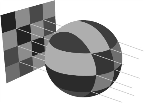
The expression fake light applies to effects applied to objects rendered in a 3-D world. However, the effects corresponding to fake light represent real-world phenomena. In this respect, then, you have ambient, directional, and attenuated light. The light striking any given point on a 3-D object is a combination of three effects. Figure 20.1 shows an object illuminated by different kinds of light.

Figure 20.1. Four different lights.

Ambient light simulates the light that surrounds you. One form of ambient light is light that has come in from a window and bounced around the room several times, until it has no real direction. It illuminates everything in the scene. In the context of a graphical simulation, since it bounces around in this way, ambient light is easy to calculate. It acts equally on all polygons in all directions. In some cases, adjustments must be made, however. For example, complex models allow the color and brightness of ambient light to vary through space.

Directional light, as the name suggests, comes from a particular direction, like the light of the sun, but it is not affected by position. It equally illuminates all objects in the scene. A scene can have any number of directional lights. For convenience, these are placed in the scene as if they were ordinary nodes, but only their rotation vector is relevant to their effect.

Attenuated light has two forms. One form is spotlight. The other form is point light. These forms of light are created by objects that can be placed in a scene to illuminate the objects around them with a particular color. Objects nearer to an attenuated light are illuminated more than those farther away. How much this happens depends on three attenuation constants that modify the brightness of the beam by a factor b. To examine how this is so, consider that for a point light you have the following equation:

On the other hand, for a spotlight pointing in the direction u and at a unit vector v with distance d from the surface, you have this equation:

where p is a special constant that measures the spread or focus of the light. A high value of p means that the light mostly illuminates a very narrow beam. A low value makes it spread out more widely. An alternative method is to specify an actual angle for the beam. You use the term max(–(u · v),0) to ensure that only surfaces whose normals point toward the light are illuminated.

A material describes all the different qualities of the surface and includes a number of different color components. The values for these qualities can be represented by either single values or image maps. Image maps are a topic covered in detail in the next section. For now, think of them as single values applied across the whole surface.

The simplest color element is called the emissive color. The emissive color is a color actually given off by the object, such as a glowing lamp. Emissive light is a cheat, however. Unlike real light, it has no effect on any other object. Instead, uniformly in all directions, it changes the color of the object emitting it. While compromising the realism of the scene, emissive light is computationally cheap and provides a simple way to create objects of different colors. You’ll designate this color with the expression C_em.

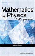
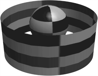
The next color element is diffuse color. Diffuse color tells you the color of light that would have a Lambertian reflectance if the surface were illuminated with full-spectrum white light. In other words, such light would be the best candidate for the color of the surface. The diffuse color does not depend on the position of the observer, but it does vary according to the angle of the light falling on the surface. As shown in Figure 20.2, since the center surface is illuminated by more of the beam, the closer the light angle is to the surface normal, the more of it is reflected.

Figure 20.2. Calculating the diffuse component.

The characteristics of surface illumination allow you to develop a formula for the diffuse color component from a surface with normal n due to a particular light. If the diffuse color of the material is d, and it’s illuminated by a light of color c from the (unit) direction v, then the Lambertian reflection c_diff is given by cd max (u · v, 0) where the multiplication of the colors is performed pairwise.

When considering the formula for Lambertian reflection, remember that color vectors are not the same as linear vectors in space. Among other things, pairwise multiplication modulates one color with another, making a blue vector more red. However, this is the correct method when dealing with a surface that absorbs some frequencies and reflects others. Note that since ambient light is normal to all surfaces, the diffuse component of an ambient light is just cd.

The specular component has two elements, a color s and an exponent m. These combine to create a light of a single color, called a specular highlight. What they don’t create is a mirror reflection. To create a mirror reflection, you must model not just the direct light on the object due to the various lights in the scene but the light reflected off all the other objects. When you pursue this objective, you enter into a raytracing territory that is computationally expensive. Given this limitation, the illumination of an object in a real-time 3-D scene is usually affected only by the lights themselves, not by light emitted, absorbed, or reflected by other objects. This outcome affects not only the possibility of mirror-images but of real-time shadows. Both of these have to be modeled in different and not entirely satisfactory ways.

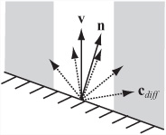
As discussed previously, a specular reflection is the light equivalent of an elastic collision. As shown in Figure 20.3, the result of this effect is that light bouncing off a surface is emitted at the same angle as it strikes the surface. The nearer the viewing vector is to this (unit) reflection vector r, the brighter the specular light becomes. You modify how near the vector needs to be by means of the exponent m, which focuses the reflection in much the same way as the exponent p focuses spotlights.

Figure 20.3. Calculating the specular component.

You can calculate the specular reflection due to a particular (non-ambient) light using different formulations. One in particular works especially well. With this approach, you assume that n · v > 0 and that the observer is at a vector w from the point on the surface. Given this understanding, you have c_spec = sc (max (r · w, 0))^m. A specular color of white is usually the most appropriate. The exponent m can take any value. A value of 0 gives you a diffuse color, and an infinitely high value gives what would in theory be a mirrored surface. In this case, only a viewing angle exactly along r will detect the light.

Each of these values needs to be calculated for each non-ambient light applied to each surface. The sum of the values due to all of the lights in the scene is the color seen by the viewer. To generate this color, you add the colors with a maximum of 1 for each primary color. You use this approach because you are combining the effects of several light sources. One color is not used to modulate another. You can sum all this up with the surfaceColor() function, which takes values corresponding to the light effects discussed in this and previous sections. This function is supplemented by others.

function surfaceColor(normal, position,
                         material, lights, observerPosition)
   set color to emissiveColor of material
   set observerVector to observerPosition - position
   
   repeat for each light in lights
      set lightColor to illumination(position, light)
      if light is not ambient then
         set v to the direction of light
         set diffuseAngle to max(-dotProd(normal, v),0)
         if diffuseAngle>0 then
            set diffuseComponent to
                      modulate(diffuseColor of material,
                                lightColor)
            add diffuseComponent*diffuseAngle to color
            
            set specularReflection to v + 2* dotProd(v, normal)
            set specularAngle to
                      max(dotProd(observerVector,
                                   specularReflection), 0)
            set brightness to power(specularAngle,
                                      specularFocus of material)
            
            set specularComponent to
                       modulate(specularColor of material, lightColor)
            add specularComponent*brightness to color

         end if
      otherwise
         add lightColor*diffuseColor of material to color
      end if
   end repeat
end function

The modulate() function attends to adjusting of colors relative to vector values:

function modulate(color1, color 2)
   return rgb(color1[1]*color2[1],
               color1[2]*color2[2], color1[3]*color2[3])
end function

The illumination() function takes parameters that define the source position of the light and the light itself.

function illumination(position, light)
   set color to the color of light
   if light is spot then
      set v to the position of light - position
      set brightnessAngle to max(-dotProd(v, direction of light), 0)
      if brightnessAngle=0 then return rgb(0,0,0)
      set brightness to power(brightnessAngle, angle factor of light)
      multiply color by brightness
   end if

   if light is spot or point then
      set d to mag(v)
      set denominator to the constant factor of light
      add the linear factor of light * d to denominator
      add the quadratic factor of light * d * d to denominator
      divide color by denominator
   end if
   return color
end function

There are additional components to materials, all of which are described by some kind of image map, which you’ll look at next.

Not all objects are a solid color. Most have some kind of detail. Detail gives a pattern or texture to objects. In order to create details, you use an image called a map. A map gives information to the 3-D API about the surface of the shape at a higher resolution than just polygon by polygon. How maps are created and projected onto the surface is discussed farther on, but for now you only need to know that they allow you to specify values for various parameters of the surface at a pixel-by-pixel level. Further, because the pixels of the image map are converted to “texels” when they are applied to the surface, you work at a texel-by-texel level. In this way, maps can be applied to different surface areas depending on how they are projected.

Some examples of image maps are as follows:

Texture, gloss, and emission maps are fairly simple to understand. Each of them is an image that gives the value of the appropriate color of a material at particular points. By specifying how the image is mapped to the surface, you can alter the end result. The process is similar to clothing a paper doll. Textures can be combined to create more complex effects in essentially the same way that they can be combined to create a complex 2-D image in a program like Adobe Photoshop. This is in addition to global diffuse, specular, and emissive components applied to the whole surface.

Calculating all the lights in a scene is the most processor-hungry part of the operation. Most of the time, you’re recalculating exactly the same values every time. And yet the lights in a scene are basically static. Given this situation, it is important to pre-calculate the lighting in the scene and save it into the texture file. This is known as baking. Baking allows you to decrease the number of real-time lights. At the same time, it also requires a significant increase in the amount of texture information.

To get around this double bind, you can create a second map, a light map. A light map defines the lighting levels for each part of the scene, usually at much lower resolution than the texture map. By using the light map to modulate the texture map, you can reuse textures across an entire scene while still gaining most of the processing advantage of an image map. Figure 20.4 shows how this works. The texture map in the first picture has been combined with the lower resolution light map in the second picture to create an image with a shadow. Most 3-D modeling software includes the option to create baked textures, both as light maps and as new complete texture maps.

Figure 20.4. Using a light map to modulate a texture map.

A bump map is a way to model variations in height at a level of detail smaller than the polygon. Examples of its use include creating pockmarks, blisters, and embossed text. Such effects are created by using shadows and highlights. The bumps are faked. The process is similar to drawing a trompe l’oeil 3-D image on a piece of paper. When the surface is viewed head-on, it’s very convincing, but you can see it’s not really 3-D when your eye is almost level with the paper.

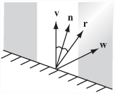
Bump maps are essentially height maps, where each point on the map represents a distance from the surface. Usually a grayscale image is employed to create the effect. An alternative is the normal map. With a normal map, by mapping the x-, y-, and z-coordinates of the (unit) vector to red, green, and blue values, each texel encodes a normal direction as a color. Ultimately, the bump map is equivalent to the normal map. The tradeoff is that with the normal map an increased amount of memory is used. With the bump map, there is a gain in performance. As shown in Figure 20.5, normal area maps are used to perturb the normal of the surface, changing the results of the directional and specular components of any lights.

Figure 20.5. A bump map and its effect on the lighting of a surface.

A normal map can be derived from a bump map. The way to do this involves how the height maps are read. With a height map, essentially, you compare the heights of pixels in small neighborhoods of the bump map.

To use your image maps correctly, you must tell the 3-D engine which part of the image corresponds to which part of the surface. To do this, you have to create a mapping from the image to the surface. In other words, for each point on the surface, you must match the point to a texel in the image map. For the sake of discussion, you can refer to this as a texture.

To match points and texels, you start by labeling your texels using standard coordinates. Textures are usually 2-D images, although for materials such as grainy wood, many people prefer to use 3-D texels, which map to the whole volume of an object and create more interesting effects. You label the texels using a separate coordinate system for clarity, such as s and t or u and v.

To map the texels to the surface, you can use a transform. You do so in a limited way, however, essentially restricting it to 2-D. However, when you do this so that you can perform scaling operations, you keep homogeneous coordinates intact. This allows you to rotate, translate, and scale the map before attaching it to each polygon. As for the mapping itself, you must still work out what to use. Some standard approaches are as follows:

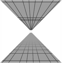
Each of these options, apart from the last, offers a way to translate the 3-D information about the points on the surface of the object into 2-D form. With a planar map, you project the 3-D coordinates of each vertex to a plane whose xy-coordinates are used to map to the st-coordinates of the texture map. As Figure 20.6 illustrates, the x- and y-coordinates of the object are mapped directly to the s- and t-coordinates of the image.

Figure 20.6. Planar mapping.

With a cylindrical map, as illustrated by Figure 20.7, you start by choosing an axis for the object. Then you calculate the distance of each vertex along the axis. This action scales the vertices to your t-coordinates. For the s-coordinate, you use the angle the vertex makes around the axis.

Figure 20.7. Cylindrical mapping.

With a spherical map, you might use the latitude and longitude of each point as projected to a sphere. Using this approach, you discard the distance from the center. This approach is shown in Figure 20.8.

Figure 20.8. Spherical mapping.

In all the cases mentioned in this section, the positions of the vertices are directly related to the texture coordinates. There are different values for these positions. You can use the object’s local geometry, or you can use its position in the world. The approach you use creates different effects. If you use the local geometry, then the texture remains the same regardless of how the model is transformed. You can rotate it, scale it, and so on, but the texture always looks the same. But if you use the world basis, the texture changes depending on how the object is placed. In particular, if you spin the object on its axis, the texture remains where it is, simulating the effect of a reflective surface. If you make a texture that represents the reflection, it will always be oriented the same way.

Reflection maps don’t always have to be used for reflections. A light map applied the same way allows your object to simulate the effect of constant shadows, like an apple turning under the dappled sunlight of a tree. You can even apply it to stranger objects, such as bump maps, but if you do this, the effect is likely to be odd. For example, lumps are likely to move around under the surface, creating an effect similar to the flesh-eating scarabs from the movie The Mummy (1999).

One problem with image maps is that the image to which they are applied may be near to or far from the camera. If the image is far away, then you’re using much more information than you need about the surface. If each pixel on the screen covers a hundred different texels, then you don’t really need to know the color of each one. In fact, having more information than you need can do more harm than good. Conversely, if the image is close, then a single texel might cover a large amount of screen space, leading to aliasing, or jagged edges between texels.

You can deal with the problem of aliasing first. When working with an object that is close to the camera, you don’t normally want to draw each texel as a solid plane of color. Instead, you want to interpolate smoothly from one to another. You can accomplish this using bilinear filtering, illustrated in Figure 20.9. Here, for each pixel, you determine the four nearest texels to a particular screen pixel and create a weighted average of all the colors at that point. In Figure 20.9, the two faces of the cube have the same 4 × 4 pixel texture. The one on the left has bilinear filtering turned on.

Figure 20.9. Bilinear filtering.

As you can see in Figure 20.9, bilinear filtering is not without its problems. It can blur the texture. One alternative technique is oversampling. With oversampling, instead of finding a single texel point under a pixel and then blurring with nearby texels, you find the texel points under a number of nearby pixels and blur them. The result is that near to the camera, you don’t see serious blurring. Instead, you see strongly delineated areas of color with nicely antialiased lines between them.

For textures at a distance, one solution is to use a mip-map, which is a set of pre-calculated textures at different levels of detail. With a mip-map, you might have a texture that is 256 × 256 texels in size but also stored in lower-resolution versions of 128 × 128 texels, 64 × 64 texels, and so on, down to 1 × 1 texels. The last version is the equivalent of the average color of the whole texture. The 3-D engine can then choose which of these maps to use depending on the amount of screen space a particular polygon takes up. The amount of memory used by the mip-mapped texture is higher than before, but not much higher. It is usually less than 50% more. The gains in both processing speed and image quality more than make up for it.

Having created your mip-maps, you still have a number of issues to deal with. For example, what happens at the transition point between different maps? If a large plane is being viewed, the nearest edge of it will be seen with the highest-quality texture map. The farther edge will be using the lowest quality. Between, there will be places where the engine switches from one map to the other, and this might be noticeable as a sudden increase in image quality. To avoid this irregularity, you can interpolate from one map to the other using trilinear filtering.

Trilinear filtering involves combining the effects of different resolutions at the boundaries. As illustrated by Figure 20.10, with such filtering, you calculate the color due to both nearby mip-maps. You then use a weighted average of the two to determine the appropriate color, smoothing the transition.

Figure 20.10. Using a mip-map, with and without trilinear filtering.

Some graphics cards use bilinear filtering. This form of filtering applies trilinear filtering selectively, usually near transition points. Some cards also use a technique called anisotropic filtering, which instead of merging square combinations of pixels, combines regions of pixels that are related to the angle of view. The result is that if the surface being viewed is heavily slanted away from the viewer, a more elongated section of it is used to create the combined pixel color. While more demanding of the processor, this approach produces a very realistic effect.

The simplest shading method is called Gouraud shading. This method of shading works by calculating the correct color at each of the three vertices of a triangle. It then interpolates them across the triangle. Gouraud shading affects only the constant components of a material. It is not affected by image maps.

The interpolation is achieved using barycentric coordinates. Barycentric coordinates are similar to homogeneous coordinates. As illustrated by the image on the left of Figure 20.11, the barycentric coordinates (w₁, w₂, w₃) of a point P in a triangle can be defined as a set of weights that can be placed at the vertices of the triangle to establish the center of gravity at P. Equivalently, they can be used to balance the triangle on a pin placed at P.

Figure 20.11. Barycentric coordinates.

If the first description of the use of barycentric coordinates in Figure 20.11 seems somewhat obscure, consider a second approach. With the second approach, picture the coordinates in terms of the three areas A, B, and C in the image on the right of Figure 20.11. You find that choosing w₁ = A, w₂ = B, and w₃ = C gives a solution to the problem. As with homogeneous coordinates, there is only one possible solution, since barycentric coordinates are invariant under scaling. As discussed in Chapter 17, since the area of a triangle is half the magnitude of the cross product of two of its sides, this gives you a simple function to calculate the barycentric coordinates of a point. The barycentric() function encapsulates the logic and mathematics of this approach:

function barycentric(p, v1, v2, v3)
   set t1 to v1-p
   set t2 to v2-p
   set t3 to v3-p
   set a1 to t1[1]*t2[2]-t1[2]*t2[1]
   set a2 to t2[1]*t3[2]-t2[2]*t3[1]
   set a3 to t3[1]*t1[2]-t3[2]*t1[1]
   return norm(vector(a1, a2, a3))
end

You can use barycentric coordinates (scaled to unit length) to interpolate colors. For each point of a triangle, you multiply each vertex color by its appropriate weight and add them together. The colorAtPoint() function accomplishes this task:

function colorAtPoint(pos, vertex1, vertex2,
                         vertex3, color1, color2, color3)
   set coords to barycentric(pos, vertex1, vertex2, vertex3)
   return color1*coords[1] + color2*coords[2] + color3*coords[3]
end function

In graphical applications, this process is made much more efficient when you employ optimizations to allow integer calculations to be used. As an added benefit, when you know the barycentric coordinates of a point, if all three coordinates are between 0 and 1, you can tell that it’s inside the triangle.

If you have a fast graphics card, you can do additional work and create a kind of global bump map for the triangle. Instead of calculating the colors and interpolating them, you interpolate the normals of the triangle and use these for pixel-by-pixel lighting calculations. This is called Phong shading. Since it is a great deal more difficult for the processor to use this approach, to save time, the 3-D engine usually interpolates, calculating the light intensity due to each light on a vertex-by-vertex basis and interpolating this across the triangle when calculating the contribution of each light.

The shading methods described in the previous section rely on calculating the normal of the smoothed surface at each vertex. This is a problem due to the processing load required. To solve this problem, consider that the normal at each vertex can be calculated in two ways. The simplest is just to calculate the mean of the normals of all triangles that share that vertex. This works well for fairly regular shapes.

A more advanced method is to weight the normal according to the size of each triangle so that more prominent triangles have a greater influence. You can do this fairly simply by using the cross product as you did in calculating barycentric coordinates.

As you’ve seen before, you find the normal to a triangle whose vertices are ordered anticlockwise as you look down on the triangle (conventionally) as v₁, v₂, v₃ by finding the normalized cross product of v₂ – v₁ and v₃ – v₁. If instead you take the non-normalized cross product, you end up with a normal whose length is twice the area of the triangle. Averaging out these vectors before normalizing gives a weighted sum as required.

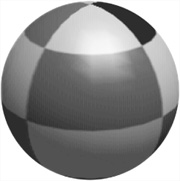
Create a function that applies a cylindrical, spherical, or planar texture map to a surface. If you have a 3-D engine, you can try the results of this function. Even without a 3-D engine, you should be able to calculate the st-coordinates for any vertex in the mesh. You’ll find the most difficult part of this problem involves dealing with the “singularities” where the texture meets itself. One such singularity is the top of the sphere.