Figure 9.1 illustrates a situation in which a ball traveling with velocity v hits a stationary, fixed wall with normal n. Since it is especially simple, this is a good example to use to explore elasticity. It is simple because you can deal with it without having to account for specific details of the ball or the wall.

Figure 9.1. A ball hitting a wall.

The simplest way to deal with the event depicted by Figure 9.1 is to split the vector v into two components, one in the direction n (the normal component) and the other in the direction of the wall (the tangential component). Because no forces act on the ball in the tangential direction, the velocity of the ball in that direction remains unchanged. In the other direction, the velocity is reversed. When looked at in this way, the energy of the ball, the only moving object in the collision, remains unchanged. The end result of this is that you can find the new velocity by simply subtracting twice the normal component. To accomplish this, consider the resolveFixedCollision() function:

function resolveFixedCollision(obj, n)
   set c to componentVector(obj.velocity, n)
   set obj.velocity to v-2*c
end function

The resolveFixedCollision() function is both simple and applies to any collision in which one of the objects is fixed in place. It makes use of componentVector() function, explained in Chapter 5. Using this function, you obtain the normal at the point of contact. With this information, you can show that the colliding object will always follow the same path. With respect to the specific workings of the function, you can try the algebra yourself. If c is the component of v in one direction, then the component in the perpendicular direction is v – c.

As is shown in Figure 9.1, a useful geometrical side effect of using the approach given by the resolveFixedCollision() function is that the angle between the original velocity vector and the wall (the angle of incidence) is equal to the angle between the final velocity vector and the wall (the angle of reflection).

As mentioned at the opening of this chapter in the discussion of elastic collisions, the calculations performed by the resolveFixedCollision() function center on the question of the ball’s motion before and after the collision. It does not address what is going on during the collision. Dealing with this problem requires a much deeper level of detail, which is dealt with in Chapter 12.

Things become more complicated when the objects are not fixed in place. If both objects can move, then you need to determine the velocity of both objects after they collide. If you consider this problem at length, one of the first things that become apparent is that you need more information.

A ball bearing hitting a cannonball is going to make a lot less difference than a wrecking ball hitting the same cannonball at the same velocity. To determine the correct solution, you need to know the masses of the two objects. More importantly, you need to know the energy and momentum of the two objects. When neither of the two objects is fixed, you have a situation in which both of the laws relating to conservation of energy apply. First, the total momentum of the two objects after a collision should be the same as the total momentum before. Second, the total energy should be equal before and after the collision.

To explore how this is so, it is easiest to begin by considering a case in which the velocity of one object before the collision is zero. As you’ll see in a moment, due to the principle of relativity, you can transform any other case to this one by subtracting one velocity from the other. Suppose you have a ball B (the incident ball) with velocity u and mass m hitting a stationary, movable ball C (the object ball) with mass p, at a normal of n. After the collision, as Figure 9.2 illustrates, B has velocity v and C has velocity w, both of which are unknown.

Figure 9.2. A collision with a stationary, movable object.

As before, you can split u into two components with magnitude u_n (normal) and u_t (tangential). The same can be done for v and w. Likewise, since the forces do not act tangentially, the velocity of each ball in the tangential direction remains unchanged. As a result, v_t = u_t and w_t = 0. In the other direction, conservation of momentum tells you that

To make calculations easier to perform later on, divide through by p to get a ratio . Using this approach, you arrive at ru_n = rv_n + w_n.

Meanwhile, conservation of energy tells you that . This equation splits up to become

Using your knowledge of the tangential direction, this becomes

You now have simultaneous equations in the unknowns v_n and w_n, which can be solved by substitution. From the momentum equation you have

Substituting this value into the energy equation, you get

Given this step, you end up with a quadratic equation in v_n, which factorizes as follows:

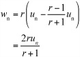
This gives you two roots of the equation: v_n = u_n and . The first of these roots is expected. It is the initial situation. The other root must represent the situation after the collision. Notice that it depends on the ratio of the masses of the balls, not on their absolute values, which makes sense physically. Also notice that the value of u_t drops out of the calculation. This, again, is to be expected. You want the two components to be completely independent.

Given the progress so far, you can now quickly determine w_n by substituting back into the momentum equation:

Having come this far, you are in a position to develop a function that addresses moving objects. This is the resolveCollisionFree1() function. As with the previous function, it makes use of the componentVector() function from Chapter 5. In this case, two objects are passed to the function, with the velocity of each altered.

function resolveCollisionFree1(obj1, obj2, n)
   set r to obj1.mass/obj2.mass
   set un to componentVector(obj1.velocity,n)
   set ut to obj1.velocity-un
   set vn to un*(r-1)/(r+1)
   set wn to un*2*r/(r+1)
   set obj1.velocity to ut+vn
   set obj2.velocity to wn
end function

Previous examples restricted you to using the velocity of one object. Adding a velocity to the second object is straightforward. To accomplish this, subtract the velocity from all objects prior to performing calculations. In effect, this makes it so that you are working with the same algorithm as before. After you subtract the velocity, remember to add it back on afterward. The resolveCollisionFree() function provides an example of this approach:

function resolveCollisionFree(obj1, obj2, n)
   set r to obj1.mass/obj2.mass
   set u to obj1.velocity-obj2.velocity
   set un to componentVector(u,n)
   set ut to u-un
   set vn to un*(r-1)/(r+1)
   set wn to un*2*r/(r+1)
   set obj1.velocity to ut+vn+u2
   set obj2.velocity to wn+u2
end function

With the resolveCollisionFree() function, except when calculating the collision normal, the shapes and sizes of the objects do not matter. This one function can handle every possible elastic collision.

There are further applications. Consider, for example, that if r = 1, the two masses are equal. If this is so, then you have v_n = 0 and w_n = u_n. This is the “Newton’s Cradle” effect, where the velocity of one ball is transferred entirely to the other. The result is that the original ball is left stationary (normal to the collision). The resolveCollisionEqualMass() function addresses this event:

function resolveCollisionEqualMass (obj1, obj2, n)
   set u to obj1.velocity-obj2.velocity
   set un to componentVector(u,n)
   set ut to u-un
   set obj1.velocity to ut+obj2.velocity
   set obj2.velocity to un+obj2.velocity
end function

With the resolveCollisionEqualMass() function, r tends to 0, then v_n → u_n and w_n → 0. In other words, the mass p tends to infinity relative to m. This is the phenomenon encountered previously with a fixed wall. When the mass of the object ball is infinite, it cannot move, so this becomes a fixed-wall collision. Conversely, when an object is fixed, it can be considered to have an infinite mass.

As you might expect given the previous discussion, with an inelastic collision, not all the initial kinetic energy existing prior to the collision is transferred to kinetic energy after the collision. A certain proportion, for example, is lost to heat or sound.

The simplest way to simulate energy loss is to establish a fixed proportion of energy that will be lost when two objects collide. This proportion is called the efficiency. Efficiency can apply to one or the other object, or to both. If the objects in your simulation are similar, you can use a global efficiency. If the objects are not similar, you are best off giving one efficiency value to each object and combining them for each collision.

For example, consider an event in which ball B, with energy, transfers 95% of its energy at each collision. Another object, ball C, transfers 90% of its energy at each collision. In a collision between the two, where B has energy E_b and C has energy E_c, the total energy after the collision is 0.95 × 0.9 × (E_b + E_c).

Like elastic collisions, this approach to inelastic collisions represents a simplification. Real collisions do not work so linearly. Generally, faster collisions are more efficient than slower ones, and efficiency is affected by factors like the ambient temperature of the surrounding air. Still, the approach remains useful, for the errors are small, especially when working within normal ranges of speed and mass.

With an inelastic collision, as mentioned previously, the equations get a bit more complicated. Fortunately, you still know that motion tangential to the collision must be unaffected. In the normal direction, conservation of momentum remains as it was before. In fact, barring external forces, this law is always true. On the other hand, conservation of energy must be revised to take efficiency into account, and you end up with this equation:

Here, the value e is the product of the efficiencies of the two objects, expressed as a fraction. You can now go through exactly the same process as before. First, putting to use your knowledge that tangential motion is unaffected, you obtain

(As before, note that ).

Substituting for w, you arrive at

Notice that this time, unless e = 1, the value of u_t does not drop out of the equation. If e = 1, perfect efficiency, then the equation reduces to the elastic example. The tangential speed does have an effect on the end result, because the more energy the system has, the more it will lose.

This equation again has two roots, which can be calculated from the quadratic formula:

The value u_n is no longer a root of the equation (unless e = 1). This is so because inelastic collisions are not time-reversible. However, by generalizing from the elastic case, you know that the particular root you are looking for is the result of taking the negative square root and substituting back for w. The result is that you can arrive at the resolveInelasticCollisionFree() function:

function resolveInelasticCollisionFree(obj1, obj2, n)
   set r to obj1.mass/obj2.mass
   set u to obj1.velocity-obj2.velocity
   set e to obj1.efficiency*obj2.efficiency
   set un to component (u,n)
   set ut to mag(u-un*n)
   set sq to r*r*un*un-(r+1)*((r-e)*un*un+(1-e)*ut*ut))
   set vn to n*(sqrt(sq)-r*un)/(r+1)
   set wn to r*(n*un-vn)
   set obj1.velocity to ut+vn+ obj2.velocity
   set obj2.velocity to wn+ obj2.velocity
end function

When e = 1, the resolveInelasticCollisionFree() function describes an elastic collision. Likewise, you can see that in this case sq = un * un, which leads to the same final values as before.

Just for completeness, the resolveInelasticCollisionFixed() function addresses fixed inelastic collisions. To reach this result, you start with the previous function and set r = 0. If you compare the resolveInelasticCollisionFixed() function to the elastic versions, you can see that they are similar.

function resolveInelasticCollisionFixed (obj1, obj2, n)
   set e to obj1.efficiency*obj2.efficiency
   set un to component (obj1.velocity,n)
   set ut to mag(obj1.velocity -un*n)
   set sq to (e*un*un+(e-1)*ut*ut))
   set vn to n*sqrt(sq)
   set obj1.velocity to ut+vn
end function

As before, the resolveInelasticCollisionFixed() function is independent of the mass of either object, which makes it much simpler to implement.

The key to complex collision detection is to understand the process involved. With respect to a computer simulation, you can break down the process into six steps:

The checkCollision() function implements this procedure. In the scope of this book, this is a long function and might be best presented as several functions. The longer approach is used to make the steps explicit. The function also includes calls to functions that depend on your computing environment. This is discussed in detail later on. Also, notice that you split the list of objects into fixed and movable, which allows you to streamline the algorithm a little.

function checkCollision(time, movableObjects, fixedObjects)
   // check for the earliest collision
   set mn to 2
   set ob1 to 0
   set ob2 to 0
   repeat for i=the number of movableObjects down to 1
      set obj1 to movableObjects[i]
      // find the displacement vector and other
      // relevant facts about this object
      set l to parameters(obj1, t)
      // search for collisions with other movableObjects
      // (don’t bother with those already checked)
      repeat for j=i-1 down to 1
         set obj2 to movableObjects[j]
         set l2 to parameters(obj2, t)
         set c to detectCollision(l,l2)
         if c is not a collision array then next repeat
         set tm to c[1] // the time of collision
         set m to min(mn,tm)
         if m<mn then
            set mn to m
            set n to c[2] // the normal vector
            set ob1 to obj1
            set ob2 to obj2
            set lf1 to l
            set lf2 to l2
         end if
      end repeat
      // now search for collisions with fixed objects
      repeat for j=the number of fixedObjects down to 1
         set obj2 to fixedObjects[j]
         set c to detectCollision(l, l2)
         if c is not a collision array then next repeat
         set tm to c[1] // the time of collision
         set m to min(mn,tm)
         if m<mn then
            set mn to m
            set n to c[2] // the normal vector
            set ob1 to obj1
            set ob2 to obj2
            set lf1 to l
            set lf2 to l2

         end if
      end repeat
   end repeat
   if mn=2 then set tmove to 1
   otherwise set tmove to mn*t
   repeat for each obj in movableObjects
      moveObject(obj, tmove)
   end repeat
   // if there is no collision you are finished
   if mn=2 then return
   // otherwise, you can resolve the collision here
   set res to resolveCollision(lf1, lf2)
   setNewVelocity(ob1, res[1])
   setNewVelocity(ob2, res[2])
   // and now recurse for the rest of the time-step
   checkCollision(t*(1-mn), movableObjects, fixedObjects)
end function

Details in the checkCollision() function have been left unfinished, because they depend on the programming environment you are working in. In an object-oriented world, each moving shape is likely to be represented by an object, probably with some kind of subclassing corresponding to different shapes. In a procedural language, you usually use an array of values for each shape. Ultimately, however, the process is the same. With respect to the functions called, while these have been dealt with previously, the specific work they perform in this context is not discussed. The implication is that specific work relative to your computing environment might be required to refine them. The goal here has been to trace the general steps.

Another point is that the function can be made much more efficient by using processes of culling. Culling involves determining beforehand which shapes are likely to collide before making calculations. In addition to culling, a further efficiency measure is to ensure that calculations that have already been performed once are not needlessly performed again. For example, in a sequence of time-step calculations, if objects A and B do not collide during one time-step, then they won’t collide in the next time-step unless struck by an object that has changed its velocity. Conversely, two objects that are about to collide during one time-step are probably going to collide at another time-step unless struck by an object that has changed its path. Generally, then, unless one of the objects that collided in the last calculation hits something, all your other calculations will remain valid. Later chapters provide further discussion of how such observations allow you to optimize your code.

Up to now, you have considered single collisions between two objects. What happens when three or more objects collide simultaneously? Consider, for example, the situation Figure 9.3 illustrates—a first ball strikes two others.

Figure 9.3. Three balls colliding simultaneously.

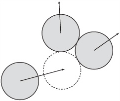
If you consider the likelihood that one object can collide with two others at precisely the same instant, you might object that this situation is extremely unlikely to occur. The implication is that the procedures for detecting single collisions, dealt with earlier in this chapter, suffice for all collisions. However, as it is, computers are not infinitely precise, and at some stage it might happen that you must deal with an exactly simultaneous collision.

The easiest way to resolve this problem is to cheat. By using a perturbation, you can alter the parameters of the simulation very slightly, forcing one of the collisions to happen first. In fact, this is implicitly the case in the existing function. It always chooses the first minimal collision encountered to be the one to resolve.

But you still need to be careful. After resolving the collision, a second will be encountered immediately, with a value of t = 0. This means that the collision time will not diminish, creating a potentially infinite loop in the function. Fortunately, in almost all situations this will not be an issue. If it were to occur, it might arise when a ball is sliding down a fixed tunnel of its exact width. Such situations can be easily avoided by not setting up your collision world so that such situations are allowed.

As shown in Figure 9.4, another example of a simultaneous collision is the Newton’s Cradle. In this instance, as shown, three balls are arranged in a row touching one another. Struck by another ball at one end with velocity v, the momentum of the incident ball passes through the group, causing the last ball to move off at the same velocity. It turns out that the same process that deals with simultaneous collisions also covers this case. B₁ is moving with velocity v, but strikes ball B₂ instantly (t = 0). The same process passes down the chain until the final ball experiences just one collision and can move off freely.

Figure 9.4. Newton’s Cradle.

Complete the checkCollision() function by filling in the missing details, particularly the two functions detectCollision() and resolveCollision().

This is mostly a programming exercise rather than a mathematical one. Try to write these functions in a general way that allows you to create new collision types and resolve them correctly.

Create a simplified Newton’s Cradle. To accomplish this, make a simulation with two fixed walls at either end, a number of touching balls in between, and one or more other balls between the group and the walls, all in a straight line. Any of the balls should be allowed to have an initial velocity along the line. See if you can use the resolution functions to make the simulation behave like a real Newton’s Cradle.