There isn’t space in this book to provide code listings for all exercises. The answers provided here are more along the lines of hints and suggestions, with some brief code snippets.
Code samples for the chapters in the book are available on the book’s companion website at www.coursePTR.com/downloads. Examples are provided, implemented in Lingo.
Exercise 1.1 To construct the convertBase(NumberString, Basel, Base2) function, the easiest way to do this (although not the most efficient) is to create one function that converts the string from base 1 to a number, and then another that converts it from a number into base 2. You can use the functions in the text for this, but look at base() and fromBase() in floats.
Exercise 1.2 Floating-point numbers. This is fairly easy until you try to deal with division. The trick is to implement a binary version of the long division algorithm: at each stage you have a current “remainder,” to which you append digits of the dividend (the number being divided) until it is greater than or equal to the divisor, at which point you subtract off the divisor, calculate the new remainder, and continue until you reach the end of the dividend. In floats, you’ll find the mantissaExponent() function, which converts a number into an IEEE-style float.
Exercise 2.1 Text scrollbar. The wording of the exercise was left deliberately vague about whether your scrollbar should be calculated according to the size of the text image, or according to the number of characters in it—that is, whether the scrollbar ratio should be “pixels/character” or “pixels/pixel.” The second is more standard (and much easier): try working on the first and see how it looks. You need to calculate how many characters are visible on the screen at any one time, in order to work out the furthest extent of your scrollbar.
Exercise 2.2 To construct the compoundinterest(amount, percentage, years) function, the key is to multiply the amount by (100 + percentage)/100 for each year.
Exercise 2.3 Slide rule function. This was a rather fancy way of saying “write a function that multiplies two numbers by summing their logarithms.” So you’re just going to use
return exp(ln(a)+ln(b))
Of course, the graphical element is just padding, but is still more complicated than this part.
Exercise 3.1, 3.2, 3.3 Solving equations. These functions are part of the same overall concept. The resource files for the book contain a rather extensive implementation of the first, substitute(), which is used by a number of other functions, although it’s worth noting that a simpler method in the function calculateValue(), which uses the Lingo keyword value, works just fine for expressions which are written in a computer-readable form. The trick to this, and all of these examples, is to use recursion extensively. For example, when simplifying an expression, you can simplify each part of it separately, and to do that you can simplify its subsidiary parts, and so on, until it’s as simple as you can make it.
Exercise 4.1 solvetriangle(triangle). Mostly this is a simple exercise in bookkeeping: there are rather a lot of different combinations of data that need to be dealt with separately. The simplest way is to try applying each of the rules (sine, cosine) in succession until you can’t apply any more.
Exercise 4.2 rotatetofollow(triangle,point). The simplest way to do this is to use some of the functions you create later in the book, such as rotateVector(). If you’re trying to do it without having read Chapter 5 and beyond and you’re struggling, then read on and it should become clearer. In a nutshell, though, you need to calculate the angles made by the lines from the centrum to the triangle vertices, as well as the angle from the centrum to point, calculate the difference between the two, and then recalculate the positions of the triangle positions using sin() and cos().
Exercise 5.1 Vector drawing. There isn’t really an “answer” to this as such. It’s just a suggestion for something to try, but you should take a look at the createA() function in Chapter 5 (vectors) and use that as your inspiration. There’s very little limit to what you can do—if you get confident, try doing the same with 3-D images.
Exercise 5.2 calculateTrajectory(oldPosition, newPosition, speed). Hopefully this should be self-explanatory. It’s something that you should always be doing in any working example.
Exercise 6.1 drawDifferentialEquation(function). If you find this difficult, then don’t be afraid: creating the one in the figure was hard work, as you can see from the solution code in Chapter 6. Having said that, most of the complexity of this matches the similar work done on other graphs, namely calculating an appropriate scale, working out how best to label the axes, and so on. The main meat of the function is just these lines:
d=calculate2DValue(functionToDraw,pt[1], pt[2])
if d=#infinite then
   p1=0
   p2=yspacing
else if d<>#undefined then
   p=point(1.0,d)
   len=sqrt(1.0+d*d)
   p=p/len
   p1=p[1]*xspacing
   p2=p[2]*yspacing
else
   next repeat
end if
Here, you are at a particular point, you draw a line from that point, then start again from the end of that line. The hardest part is creating a reasonable spread of lines, which is solved by the rather cheeky expedient of simply choosing a number of random start points and seeing where they take you.
Exercise 6.2 secantMethod(). This is a fairly simple extension of the examples in the chapter. This function is designed to be as fast as possible, which is done by caching as many reference values as you can make use of.
Exercise 7.1 javelin(throwAngle, throwSpeed, time). The key trick is to calculate the velocity vector at each stage, and then rotate the javelin to follow it. Notice that the code also includes some simple collision-detection mechanisms to determine when the javelin reaches the edge of the screen (although it’s allowed to go off the top).
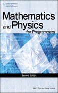
Exercise 7.2 aimCannon(cannonLength, muzzleSpeed, aimPoint). This exercise was included as something of a trick, because it’s not at all an easy calculation. Here is how you might work through it:
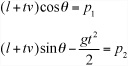
Suppose the cannon has length l and speed v, and you’re trying to hit the point with position vector p. The ball leaves the cannon from the point with speed v, so at time t its position is
So you are solving
Now, there are a number of possible approaches to this. It is solvable directly (substituting for sin θ in the second equation yields a quartic equation in t, which can be solved algebraically), but it’s really easier to use an approximation method to approach the solution iteratively.
You can start by creating a function that tests whether the current aim is high or low (by working out the ball’s y position when its x position is p1). This function should return 1 for high, –1 for low, and 0 for a hit or close to it. Notice first of all that if you aim the cannon directly at the target point, it will always fall short. If you use this angle as your baseline, then work up in increments until you find a firing angle that is aiming high. You can then use a simple binary approximation method to find the solution.
Exercise 7.3 fireCannon(massOfBall, massOfCannon, energy). This should be a straightforward application of the formulas in the chapter.
Exercise 8.1 pointParallelogramCollision(pt, parr, tm). The chapter suggests using a skew transformation to turn the parallelogram into a normal rectangle. If you would prefer to solve the problem directly, you can represent it as a collision with four separate walls: you can work out which two walls are potential collision material by finding the dot product of their normals with the particle velocity, and then use the usual methods to determine which of them collide.
Exercise 8.2 Inner collisions. Generally, inner collisions are simpler to deal with than outer ones. For example, a rectangle inside a circle can only collide at its vertices, while a circle inside a rectangle can never collide with a vertex, and a rectangle inside a rectangle can only collide at a vertex if they are axis-aligned.
Exercise 9.1 checkCollision(). This is a tricky thing to do in abstract. You might find that without creating a generic collision detection environment, you can’t really test how well it’s working. But the version in the chapter includes quite a lot of detail, so keep trying.
Exercise 9.2 Newton’s Cradle. Depending on how simplified you want this to be, it can be either very easy or extremely difficult. The goal in this context is to keep it simple.
Exercise 10.1 splitPolygon(poly). As suggested in the chapter, this is best done recursively: choose three adjacent vertices, check if the third line of their triangle intersects with any others in the shape, and if so, split it off.
Exercise 10.2 smoothNormals(collisionMap). This is found in the chapter’s discussion of object modeling and collisions. At each step, the function checks through all the pixels of the collision map, and for any edge pixel it finds any adjacent pixels and sets the normal to the average of adjacent pixels. After about four iterations, you get a very close fit to the surface.
Exercise 11.1 Checking for a pocketed ball. If the ball passes between the pocket jaws, it will intersect the circle defining the pocket, so this should be foolproof, although it never seems very elegant. Another method would be to check against a line drawn along the pocket entrance.
Exercise 11.2 Ball preview. This is easier to do than you might think. The trick is to perform a regular collision detection, but with an extremely high “velocity.” When you’ve found your first collision, you can calculate its resolution and draw the result into your image.
Exercise 12.1 Worlds in collision. As noted in the chapter, the simulation is only of limited success because of problems of scale. Nevertheless, it works as far as it goes.
Exercise 13.1 resolveCushionCollision(obj1, obj2, normal, moment, slow). Review the notes in the chapter.
Exercise 13.2 A moving, rotating square and a wall. This is a tricky problem but not insurmountable. Since you don’t need to deal with the ends of the wall, the only possible collision is between the vertices of the square and the wall. You can calculate this to a precise degree of accuracy by an approximation method, but really this is a good example of a case where it’s easiest just to calculate whether any vertex of the square starts on one side of the wall and ends up on the other. The result will be close enough for any common purpose.
Exercise 14.1 applyFriction(velocity, topSpin, radius, mass, muK, muS, time). Although fairly straightforward, this is something of a drop in the ocean where implementing spin fully in the pool game is concerned. The real difficulty is dealing with how to calculate the topspin in the first place. As soon as the ball changes direction, it is spinning at a strange angle compared to the direction of travel, and this complicates things quite a bit. Your pool simulation cheats: you might like to think about how to do things more realistically.
Exercise 15.1 Rockets. This one should be pure book work.
Exercise 16.1 Springs. You’ll find that the versions quite quickly start to behave differently as a result of calculation errors. The hardest thing to get right is the elastic limit, and this code doesn’t quite achieve it.
Exercise 17.1 Drawing a 3-D cube and culling the back faces. The way you do this is quite simple. You don’t draw any face whose outward normal is pointing away from you. Such a face has a positive dot product with the vector from the camera to the face. In a wireframe drawing, you can work on a vertex-by-vertex basis: a vertex is culled if all faces sharing that vertex are facing backward. Then you only draw lines both of whose vertices are visible. The next step in this code would be to create z-ordering—that is, to draw objects nearer to the camera in front of those farther away.
Exercise 18.1 Applying relative transforms. These can be found in Chapter 18. They should be straightforward enough.
Exercise 19.1 3-D collisions. The exercise didn’t specify which collision to implement, as by now you should be used to the formula. At the very least, you should find spheres and planes reasonably simple.
Exercise 20.1 Texture maps. There’s a lot involved in creating the mesh, but you only really need to look at the lines involving the textureCoordinates property.
Exercise 21.1 2-D NURBS. The implementation is fairly simple if you just follow the equations in the chapter.
Exercise 21.2 IKapproach(chain, target). The trick with this is to work backward: start by adjusting the most central limb to rotate it toward the target, then adjust the next one out, and so on until you get to the last bone.
Exercise 22.1 Complete drawBresenham(). This can be found in Chapter 22. It should be a simple extension of the function in the chapter.
Exercise 22.2 Car control. One of the great goals of pseudo-physics is, “How simple can this be and still feel complicated?” The aim here is to get the perfect balance between simplicity and complexity.
Exercise 23.1 box3DTileTopCollision(). This is a difficult problem. It is more difficult if you try it with a non-aligned box.
Exercise 24.1 Maze navigation. Consider what is involved in recursive backtracking for maze creation.
Exercise 25.1 Heads or tails. Few approaches improve over the one that is most basic.
Exercise 25.2 Boids. Boid rules are well-documented, so if you have trouble with this, you might want to do some research online. Try Craig Reynolds’ own site (www.red3d.com/cwr/boids) to start with; it’s well worth a visit.
Exercise 26.1 Eight queens genetic algorithm. The demo geneticAlgorithm() function shows one approach to this. This includes a system of varying radiation to speed things up a little. (It also demonstrates some examples of how you can keep tabs on your program’s performance when running this kind of extended search.)