The length of time an algorithm takes is called its computational complexity. Computational complexity is expressed in terms of the size of the function arguments. For example, while the process of incrementing a number stored on the computer by 1 is essentially independent of the size of the number, it would be pointless to use this method to add two numbers together:

function sillyAdd(n1, n2)
   repeat for i=1 to n1
      add 1 to n2
   end repeat
   return n2
end function

The length of time this algorithm takes is roughly proportional to the size of n1. As this value becomes very large, the length of time for simple operations like storing the value n2 and returning the answer becomes increasingly irrelevant. In this respect, the algorithm is linear, and as a linear algorithm it has an order of 1. To express that an algorithm has a given order, you write O(n), with n indicating the order.

A much more efficient algorithm for adding two numbers is the method usually presented in school. This algorithm takes the binary form discussed in Chapter 1. With this approach, if you assume that n2 is fixed, the time taken by the algorithm mostly depends on the number of digits in the binary representation of n1, which is roughly proportional to the logarithm of the number. You say, then, that the algorithm is O(log(n)). The larger your numbers get, the faster this algorithm is in comparison to the sillyAdd() function.

The following list identifies a few of the most common kinds of algorithm:

A few notes might be added to the preceding discussion. The base of the logarithm might be important for small values in a function, but it might also become irrelevant when dealing with very large numbers. What applies to mathematics alone might not apply to dealing with practical computations. Practical computations are just as likely to involve small numbers as large ones. If your function is proportional to 1,000,000n, for example, and you are comparing it to another that is proportional to n², then computational efficiency is important. For smaller numbers, however, the efficiency of the algorithm might not be important at all.

What applies to computational complexity also applies to benchmark tests. With a benchmark test, a particular calculation is run a large number of times with different methods in order to evaluate the speed of the calculation. Benchmarks need to be considered carefully in order to put them into context. After all, how often do you need to perform the same calculation a million times in succession? Usually, a calculation is a part of a larger process, and this can affect the value of the different algorithms. For example, one process might be significantly faster but involve higher memory usage. Such situations arise commonly since one of the principal ways to speed up calculations is to use look-up tables. Another process might take slightly longer but produce a number of other intermediate values that are useful later on and reduce the time taken by another process.

When dealing with computationally expensive calculations, one solution is to use a look-up table. A look-up table is a list of values of a given function pre-calculated over a given range of inputs. A common example is the trigonometric functions. Instead of calculating sin(x) directly, you can look it up from the table by finding the nearest entries to x in the table and interpolating between them. For the trigonometric functions, you can use some optimizations to limit the number of entries, since you only need the values of sin(x) from 0 to π/2 to calculate the complete list of entries for sine, cosine, and tangent. You can also use the table in reverse to find the inverse functions.

How many entries a table needs to contain depends on how accurate the look-up needs to be. It also depends on the interpolation method. A linear interpolation is quicker but requires more memory while a cubic interpolation, such as one based on the same principle as the Catmull-Rom splines mentioned in Chapter 10, uses fewer points but requires a little more processing. The difference is fairly significant. With no more than 15 control points, you can use cubic interpolation to calculate the values of sin(x) to an accuracy of four decimal places. (To save on calculation, you can store 15 × 4 = 60 cubic coefficients.) Using linear interpolation, you need well over 200 points to get the same degree of accuracy. Two hundred points with cubic interpolation is accurate to seven decimal places.

Although look-up tables can save some time, it’s worth considering that the engine powering your programming language almost certainly uses a look-up table of its own to calculate such values. If you want to calculate the trigonometric, logarithmic, or exponential functions to a high degree of accuracy, it’s almost certainly going to be quicker just to use the inbuilt calculations. Look-up tables are only useful if you’re willing to drop some information. If you’re willing to drop a great deal of information, you can ignore the interpolation step altogether and simply find the nearest point in your table.

In addition to calculating standard values, you can use a bespoke look-up table for your own special purposes. A common example of a bespoke look-up table is one that is used for a character and some kind of jump function. Consider, for example, the actions of a character in a platform game. Instead of calculating the motion through the air using ballistic physics each time the character jumps, you can pre-calculate the list of heights. In addition to the speed advantages, this also helps to standardize the motion across different times and machines.

As was discussed in Chapter 1, it’s significantly faster to use integer values for calculations than floating-point values. Although for simplicity you’ve mostly ignored this issue, it’s often possible to improve the speed of an algorithm by replacing floats with integers. In the simplest example, instead of finding a value as a float between 0 and 1, you find the value as an integer between, say, 1 and 1000. You can then scale all other calculations accordingly.

However, there is a problem with the integer-scaling approach. The problem arises with rounding errors. The errors that accumulate when performing multiple calculations with floats are even more prevalent when you are restricted to integers. As a result, you have to be quite clever in order to ensure that accuracy is maintained. Achieving accuracy generally means finding algorithms that rely only on initial data and not building calculations on intermediate values.

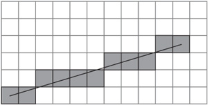
Achieving accuracy by using initial data and avoiding intermediate values can be explained most readily by means of a concrete example. Figure 22.1 illustrates a common problem scenario. In this illustration, a board is set up with a set of squares arranged uniformly. Suppose that you want to move from A to B along a grid of squares. You want to find the set of squares that most closely approximates a straight line. This is the problem that painting software faces every time it draws a line as a sequence of pixels with no gaps.

Figure 22.1. Approximating a straight line on a square grid.

The best method known for addressing the grid problem involves Bresenham’s Algorithm. Figure 22.2 illustrates how Bresenham’s Algorithm works. Suppose you are drawing a line between two points P₁ = (x₁, y₁) and P₂ = (x₂, y₂). Say for the sake of argument that x₂ > x₁, that all the values are integers, and that the gradient m of the line, measuring y downward, is between 0 and –1. (In the end, adjustments will be made to these assumptions.)

Figure 22.2. Bresenham’s Algorithm.

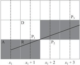
Figure 22.2 focuses on the start of the line. The pixel at point A is filled in, and because of your assumptions about the gradient of the line, you know that the next point you’re interested in is either the next pixel to the right (R) or the pixel diagonally upward (D). Which one you want to fill in depends on the slope of the line. In particular, you are interested in whether the point marked P₁, above the point x₁ + 1, lies above or below the line between R and D.

You can continue this process of determining which square to fill in on a step-by-step basis, moving either right or diagonally at each point, depending on whether your line at the midpoint is above or below the half-way line. The squares you will fill in are lightly shaded in the figure. All you need is an efficient way to calculate whether the line is above or below your test position at each step such that only integer values are involved.

You can rewrite m as , where a = y₂ – y₁ and b = x₂ – x₁. Note that a and b are both integers. Then your line equation y = mx + c becomes by – ax – bc = 0, with bc found by substituting the coordinates of A into this equation, so bc – by₁ – ax₁. Given this start, you can define a function L(x, y) = by – ax – bc. For any point (x, y) above the line, L(x, y) < 0, and for any point below the line, L(x, y) > 0.

You are now in a position to create an iterative method of solution, which is the opposite of a recursive algorithm. An iterative algorithm works by defining two elements. The first element is what you do on the first step. The second element is how you get from any particular step to a subsequent step. For example, an iterative algorithm for climbing a flight of stairs might be “go to the bottom of the first step; then for each step, walk onto the next step until you reach the top.” In this case, you create a series of midpoints given by P₁, P₂, p₁, ..., each of which is determined based on the previous one. For each midpoint, you calculate the value of L(P_i+1) based on the value of L(P_i).

Now consider the first step, where you are moving from (x₁, y₁). In this case, the midpoint you’re interested in is P₁ = (x₁ + 1, y₁ – ), and you want to know if L(P₁) = by₁ – – ax₁ – a – bc < 0. Substituting in the value of bc, you get L(P₁) = by₁ – – a. To keep everything in integers, you can multiply the inequality by 2 (which does not affect the result). If the inequality is true, then you move diagonally; otherwise, you move right.

Now that you know this, you can think of what you do at each further step. With reference to Figure 22.2, the situation breaks down into two cases. If at the previous step you moved right, then the midpoint you’re interested in has the same y-coordinate as before but an x-coordinate that is one greater. If you moved diagonally, then the y-coordinate must decrease by 1.

In the first case, if the last midpoint (P_i) you checked had coordinates (x_i, y_i) and you moved right, then you know that P_i+1 = (x_i + 1, y_i), so you move right again if L(x_i + 1, y_i) < 0. Otherwise, you move diagonally. This gives the inequality by_i – ax_i – a – bc < 0. Notice that this is the same as L(x_i, y_i) – a < 0. In the second case, having moved diagonally, P_i+1 = (x_i + 1, y_i – 1), you have by_i – b – ax_i – a – bc < 0, or L(x_i, y_i) – a – b < 0. Again, you multiply everything by 2 to ensure that you are still in integer territory.

The drawBresenham() function encapsulates this reasoning:

function drawBresenham(startCoords, endCoords)
   drawPixel(startCoords)
   set x to startCoords[1]
   set y to startCoords[2]
   set a to endCoords[1]-x
   set b to endCoords[2]-y
   set d to 2*(a+b)
   set e to 2*a
   // calculate 2L(P1)
   set linefn to -2*a-b

   // perform iteration
   repeat for x=x+1 to endcoords[1]
      if linefn<0 then // move diagonally
         subtract 1 from y
         subtract d from linefn
      otherwise // move right
         add e to linefn
      end if
      drawPixel(x,y)
   end repeat
end function

The code given for the drawBresenham() function must be adapted to deal with the other cases, where the absolute value of the gradient is greater than 1. In such a case, you must switch x and y in the algorithm. In another case, the value of the gradient might be positive, and you must add 1 to y at each stage instead of subtracting and switch the sign of a. If the x-coordinate of the start point is greater than that of the end point, you can just switch the two points around. Exercise 22.1 challenges you to deal with such changes.

Exploration of Bresenham’s Algorithm and the drawBresenham() function provides a good approach to understanding the principles of integer calculations. In particular, it shows you the process of approximating to integers efficiently so that you do not lose original detail. The Bresenham Algorithm is also useful in its own right, not just in drawing, but also in pathfinding, motion, and collision detection. It allows you to digitalize a world with complex lines and angles into a more tractable and faster form.

As you’ve already seen, calculating collisions can get fairly unpleasant fairly quickly. Even a simple problem like finding the point of collision between two ellipses or a circle and a rotating line leads to situations that require a numerical solution. Numerical solutions are usually computationally expensive.

If your time slices are small enough, you can fake collisions to a reasonable degree of accuracy using a simple process. The faking involves two steps. First, you find out whether a collision has occurred during a particular time slice. Next, you make a guess as to when it happened. In most cases, this process is not too hard to implement and produces a fairly believable effect. While there are a few potential pitfalls, you can mostly get around them.

To examine a simple example, consider the collision of two ellipses. You can reduce the collision of two ellipses to the collision of one ellipse aligned along the x-axis with a unit circle. Suppose, then, that you have an ellipse E(p, (1 0)^T, a, b) moving along a displacement vector v, and you want to see if it collides with the circle C(0,1).

If your time slice is small enough, then for the ellipse to collide during this time period, it must intersect the circle at the end of the time designated. If it doesn’t, then the only way it can collide is if it glances off the circle at a very shallow angle. The angle can be ignored since such collisions don’t have much effect.

Deciding if there is a (pseudo-)collision is essentially the same as calculating if the ellipse intersects with C. In other words, you are looking for a point on at a distance less than 1 from the origin:

where q = p + v. You can carry out this operation by searching for the minimum value of this expression. You find the minimum value by differentiating and setting the derivative to 0:

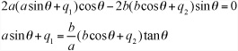
Substituting this back into the inequality, you are looking for

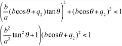
Given that , with a little algebraic manipulation, you end up with the following quartic inequality:

Where c = cosθ. You can solve this inequality algebraically. If it yields a value of c between –1 and 1, you know that a collision occurs.

You can make similar simplifications when dealing with rotational motion. For example, collisions between two moving objects that are spinning can be calculated by ignoring the spin. At each stage, you calculate a linear collision between the objects in their current orientation. This will not work, however, when neither object is moving linearly. Likewise, you will miss some collisions on the fringes, where they are less noticeable.

Pseudo-physics can be used to deal with several other types of motion. One of these is friction. In the pool game explored in previous chapters, you implemented a simple system of pseudo-friction in which the balls slowed down at a constant rate. As a general rule, you can simplify things roughly in proportion to how attuned people are to them. If your simulation is for people who possess a very accurate intuition about objects in flight, for example, then the ballistics of your simulation must be implemented accurately. On the other hand, the intuitive understanding most people have of oscillations is usually not very strong, so you are not likely to encounter strong objections if you present a fairly rough simulation of objects on springs. An example would be applying a uniform backward acceleration whenever a spring is extended, combined, perhaps, with a uniform frictional deceleration applied at all times.

Similarly, most people have a natural understanding of linear momentum and energy but tend to be weak with respect to their understanding of angular motion. For this reason, it is predictable that many people find some of the phenomena associated with spin strange or magical. For this reason, you are taking few risks if you significantly simplify angular motion. An example in this respect is resolving a spinning collision by applying an additional impulse in the direction of spin instead of accurately resolving the angular and linear components.

In most game contexts, people are often more comfortable with pseudo-physics than with highly precise physical simulations. Consider an automobile racing game. If such a game uses realistic physics for driving a racing car or a four-by-four, it is likely the user will find the vehicles much harder to control than if they are governed by simplified, discrete motion. Such motion applies to forward, backward, left, and right movements. Due in part to gameplay satisfaction, game designers have, as a rule, differed on whether it is essential to make real-time physics a genuine part of the game. What happens, for example, if the difficulty of your game were to make it impossible for the majority of your potential customers to win? Exercise 22.2 asks you to explore this topic further.

Recall that in Chapter 11 you explored techniques for partitioning or segregating the game world into smaller chunks. This technique can be generalized in two ways. One is to make the chunks smaller and tie them in to the actual game world design, which leads to the tile-based games you’ll examine in the next chapter. The other is to create a recursive process that organizes the world into regions within regions, creating a partitioning tree. In this section, a number of methods for developing partitioning trees are discussed. All of these methods work equally well in two or three dimensions, but the discussion concentrates on 2-D examples because you rarely need a 3-D implementation of them. Three-dimensional games tend to take place on a ground of some kind, making them essentially 2-D (or 2.5-D). Only a few games, such as space battles, fully use three dimensions.

A partitioning tree is a data structure that stores information about the world in some form of hierarchy. The form of the tree is essentially the same as the system used in Chapter 18 to deal with relative parent-child transforms. It consists of a number of nodes, all but one of which has a single parent and zero or more children. A childless node is called a leaf, and the topmost, parentless node is called the root. As you might infer from the discussion presented here, trees are generally drawn upside down. A tree contains no loops. No node can be its own parent, grandparent, or other relative. Information used to make calculations is associated with each node, and in this realm, you require an understanding of object-oriented programming.

In a partitioning tree, the root node represents the whole world, which is then split into smaller (generally non-overlapping) parts based on some criterion. These parts are then split again, and again, and so on, until some pre-set condition is reached, such as a minimum size. The partition is usually performed in such a way that calculations such as raycasting or collision detection are simplified. In particular, if something is not true of a parent node (visibility, proximity, and so on), then it is not true of any of the parent’s children, which means that you need not bother checking any further along the branch of the tree associated with the parent node.

As was pointed out in Chapter 11, partitioning trees can’t solve all ills and shouldn’t be expected to. For example, checking each parent node in itself adds an additional calculation. If you happen to be looking toward every object in the world, then you’re going to be performing all your visibility culling calculations for nothing. Similarly, if you’re performing a break in a game of pool, you can’t avoid the fact that every ball on the table is involved and has to be checked. Nevertheless, in many circumstances partitioning space is helpful, and in some cases, such as working on a vast outdoor terrain, it is essential.

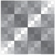
Probably the simplest and most common form of partitioning tree is the quadtree, or its 3-D equivalent, the octree. A quadtree is the most natural extension of the system you looked at in the pool game, in which the world is broken up into square regions. Suppose you start with one large square that encompasses the whole 2-D plane. This is the root node. You can break up the root node into four equal squares, which are its children. Each of the children in turn, can be broken into four smaller squares. As shown in the tartan in Figure 22.3, the process of breaking up child nodes can continue until your squares are a pre-set minimum size.

Figure 22.3. A 2-D plane broken into a quadtree.

Associated with each leaf node is the set of objects contained in the node’s area, which might be either complete geometrical objects, such as balls, or individual line segments of a polygon. (With a 3-D mesh, multiple polygons would be used.) Objects in more than one square are associated with all these leaves. Associated with each parent node is its set of vertices on the plane and, possibly, a duplicate set of all the objects it contains.

Various algorithms for searching a tree have been developed, dealing with a variety of problems. To examine one example of searching a tree, consider collision detection. When detecting objects that are colliding, for each object you cull out any parent nodes whose partition does not contain any part of the object’s trajectory during a given time slice. As shown in Figure 22.4, you begin by removing the partitions shaded with the darkest gray. Next, you remove the children shaded with the next darkest. The process continues, until you end up with a set of leaves that intersect the motion. You can then quickly check for collisions with any objects in these leaves.

Figure 22.4. Culling for collision detection with a quadtree.

Despite the simplicity of this algorithm, it is not significantly quicker than just partitioning the space into a flat grid. In some circumstances, it can even be slower. However, to speed things up, you can pre-compute sets of nodes that can be culled automatically for an object in a given leaf. If the amount of motion is small relative to the size of the grid, you can assume that an object in the middle of a first-level partition can’t ever get to one of the other first-level nodes. While effective generally, this approach won’t work for nodes on the edges of a particular parent.

Quadtrees are useful for visibility determination because they allow you to reduce the number of leaves you need to consider in your calculations. They also can be useful for raycasting. With raycasting, you can determine the set of parent nodes intersecting with a ray. If a parent node is known to be empty, then you can ignore it; otherwise, you recurse over its children. One project worth attempting is to adapt Bresenham’s Algorithm to perform this operation using a fast integer-only algorithm.

At the object level, quadtrees are most useful for storing a collision map. Figure 22.5 illustrates a collision map that has been divided into a quadtree using the following algorithm: If a particular partition is either completely empty or completely full (partitions A and B, for example), you stop subdividing the tree at that stage; otherwise, you recurse over its children. You can further optimize this algorithm by stopping whenever a particular node contains a flat edge. When detecting collisions between such shapes, you work down through the nodes of the trees until either a collision is detected (a black leaf from each shape intersects) or all nodes at that level in one or another shape are empty.

Figure 22.5. A collision map organized as a quadtree.

A second type of partition is the binary space partitioning tree, or BSP tree. Unlike quadtrees, BSP trees use two children for each non-leaf node, so each partition is divided into two parts at each stage, either by a line in 2-D or a plane in 3-D. You can choose various approaches to making the partition. One method of accomplishing this involves making each leaf node contain exactly one object, as is illustrated by Figure 22.6. The object might be one line segment or polygon. A common technique is to use a split line oriented along a particular line segment or polygon of the partitioned region. Using this approach means that your BSP tree has to be recalculated every time an object moves out of its current partition. For this reason, this kind of tree is best suited for a scene that is mostly static. Each node of the BSP tree keeps a record of all objects that are entirely contained within it.

Figure 22.6. A binary partition of a plane.

One useful feature of a BSP tree is that all the regions are convex. For this reason, a BSP tree provides a neat way to divide a concave object into convex parts. As with quadtrees, BSP trees are best suited at the world level and to working with visibility and raycasting. At the object level, they can also be helpful for detecting object-to-object collisions.

A bounding volume hierarchy, or BVH, is in some ways the opposite of the space partitions examined so far. Instead of concentrating on space, a BVH focuses on the objects and organizes them according to bounding shapes. The BVH is most commonly used in complex 3-D worlds, but it is equally applicable to 2-D. The bounding shapes might be spheres, AABBs, OABBs, or any other useful armature.

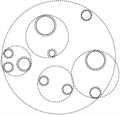
The crucial difference between this approach and those discussed previously is that a BVH does not in general cover the whole game world. It does not do so because large regions of empty space are likely to be outside the bounding volumes and, on the other hand, its various volumes can overlap. Figure 22.7 shows an example of a 2-D bounding area hierarchy in which the bounding shapes are circles.

Figure 22.7. A 2-D bounding area hierarchy for segregating a space.

BVHs are an extremely useful tool for culling and have a number of advantages over other systems, particularly in a game world made up of many moving objects. They can also be combined with space partitioning systems in various ways.

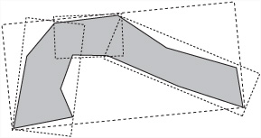
The most difficult part of working with a BVH is constructing the tree in the first place. Since you want it to be as efficient as possible, at each level of the tree, you make the bounding volumes as small as possible. Depending on the way your game is constructed, you can choose a number of different systems. In particular, objects that generally appear together should be grouped together. Objects that are moving relative to one another should not be grouped together. Within an object, you can also create a hierarchy of bounding volumes that gradually approaches the shape of the object. Figure 22.8 shows an object surrounded by a hierarchy of smaller bounding OABBs.

Figure 22.8. Using a BVH to whittle down the geometry of a shape.

When objects are moving significantly relative to one another, you must create a more dynamic BVH. Creating a more dynamic BVH involves quickly splitting, merging, and inserting new nodes in the tree. This is a complex process, but a great deal of work has been done on the subject, and it is worth looking into if you want to explore partitioning tree systems further, particularly if you are dealing with a large, complex world.

In addition to the techniques mentioned in this chapter, keep in mind that there are other systems of culling. Among many are those using visibility graphs, which store details for visible areas. Investing the available technologies amounts to an extended task that can end up leading you into a very specialized line of work. Hopefully, this taster gives you some insight into the tricks of this very interesting trade. Further references can be found in Appendix D.

Complete the drawBresenham() function by extending it to deal with all possible gradients. Some hints as to how to complete this exercise are given in the description of the function.

Write a function that controls a car with the cursor keys using simplified physics. The standard car-control system used in most games employs the up and down arrows to accelerate and brake and the left and right arrows to turn. The orientation is in the forward direction, so a left turn makes you point right if you’re moving backward. If you have the urge, you might want to extend this with a skid option. If the momentum perpendicular to the forward direction is above some threshold, then the turn function ceases to be effective.