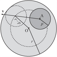
You’ve looked at circles in previous chapters. A circle is the set of points equidistant from a particular point. The particular point is the center, O, of the circle. The distance from the circumference to the center is the radius of the circle. The vector from O to any point P on the circumference is given by for some angle . The tangent of a circle at P is perpendicular to the radius . It is convenient to use the notation C(o, r) to indicate a circle of radius r centered on the point with position vector o.

It is easy to tell if a point P is inside a circle. All you do is calculate the distance OP and compare it to the radius. If the distance is less than the radius, the point is inside; if is not less than the radius, then it is outside. If it is equal to the radius, the point is on the circumference.

One more useful fact is that if two circles with centers O and O’ are touching at a point P, the points O, P, O’ are collinear. This follows directly from the fact that the tangent at P is perpendicular to both and . Remembering this relationship helps you to solve collision problems geometrically.

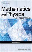
As illustrated in Figure 8.1a, to deal with a moving circle and a wall, you can start with a circle C(o, r) moving at some velocity v toward a straight line. Consider, for example, the game of Pong.

Figure 8.1. A circle moving toward a wall (a) at its start position and (b) touching the wall.

Given the time step illustrated by Figure 8.1a, you know the position O of the center of C at time 0. You also know a point A with position vector a on the line. Additionally, you know a vector w along the line. (For now, assume that the wall is infinitely long.) Given particular values for v, w, o, a, and r, two questions then arise. Will the circle hit the wall during this time-step? If so, when?

Assuming it hits the wall, in Figure 8.1b, you can see the circle C at the point of impact. The circle C is touching the wall at a point P, and the center is now at O’. You know that is perpendicular to w since the wall must be a tangent to C at P. What’s more, since it is the vector along which C has moved, you know that is some multiple of v.

So what can you deduce from this information? Do you have all that you require to define a function for collision detection? To answer these questions, start with , which can be called, tentatively, vector r. You know that r is perpendicular to w and that its length is r. All you need to derive is the direction in which it points. You can work this out using the vector . To do so, take either of the two unit normals to w and call it n. If the angle between n and is greater than 90°, then n is basically pointing toward O, and r = rn. If the angle is less than 90°, then n is pointing away from the circle, and r = -rn. To distinguish between these possibilities, take the dot product of n and . This identifies the component of in the direction n. If the absolute value of this component is less than r, then the circle becomes embedded in the wall and your function should return an error.

After you have calculated n, you can also make another quick check. If the dot product of v and n is positive, the circle is already moving away from the wall. In this situation, no collision occurs. Otherwise, you now have a simple vector equation. You know that P is on AB and that it is a vector r away from a point on the trajectory of O. For the scalars s and t, this gives you the equation

Having derived this equation, you can create the circleWallCollision() function, which detects the collision of the circle and the wall. Here is the pseudocode for the function. Again, note that object-oriented syntax is used to indicate the properties of the circle and wall objects:

function circleWallCollision(cir, wal)
   // calculate the normal to the wall
   set n to wal.normal
   set a to wal.startPoint-cir.pos
   set c to dotProduct(a, n)
   if abs(c)<cir.radius then return "embedded"
   if c<0 then set r to n*radius
   otherwise set r to -n*radius
   

   // check if the circle is approaching the wall
   set v to dotProduct(displacement, n)
   if v>0 then return "none"
   

   // calculate the vector equation
   set p to cir.pos+r
   set t to intersectionTime(cir.pos,
                    cir.displacement,
                    wal.startPoint,
                    wal.vector) // see Chapter 5
   if t>1 then return "none"
   return t
end function

The code in the circleWallCollision() function makes use of functions discussed in Chapter 5. (Review Chapter 5 for extended details.) However, with reference to the call to the intersectionTime() function, the arguments you supply are p1, v1, p2, v2. The function returns the proportion t of v1 from p1 that must be traveled before you meet the line from p2 along the vector v2. As discussed in Chapter 5, you can draw some helpful conclusions about the intersection point from this value. For example, if t lies on [0,1], an intersection occurs within the time period you are interested in. Given this frame of reference, if the circle is approaching the wall, t will always be greater than or equal to 0. This concept arises often throughout this and following chapters.

Another case concerning collisions with circles involves small objects, such as a point particle moving through space. In this scenario, your objective is to determine if the point collides with a circle in the same space occupied by the circle.

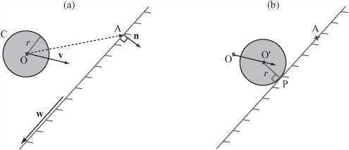
As you have already seen, determining if a point is inside a circle is trivial. To deal with the question at hand, you need to determine when, if ever, the particle’s trajectory enters the radius of the circle. In Figure 8.2, you can see an example of this. In this case, in addition to the position P and vector v of the point, you know the position O and radius r of the circle.

Figure 8.2. A stationary circle and a moving point.

To solve this problem of where the point lies with relation to the circle, look at the point Q in Figure 8.2. This is where the particle enters the circle. The point Q lies on the circle C, but it is also on the trajectory of the particle. Its position vector is given by p + tv for some t, and also the magnitude of the vector from this point to O is r. With this information, you can derive the following vector equation:

Because you know all of these values except t, this equation is fairly easy to solve. You multiply out the brackets and see what you get. (Note that the name w is given to the vector p – o.) Working through the multiplication, you end up with the following formulation:

While this is a fairly involved formula, it remains that it has resulted from simple calculations, and you can deduce that if t is less than 0, the point is moving away from C. Likewise, if t is greater than 1, the point will not hit C in this time-step. Finally, if t is imaginary—if the value under the square root is less than zero—then the trajectory doesn’t meet the circle at all. To make use of the calculation, you can develop the pointCircleCollision() function.

function pointCircleCollision(pt, cir)
    set w to pt.pos-cir.pos
    set ww to dotProduct(w,w)
    if ww<cir.radius*cir.radius then return "inside"
    set v to pt.displacement-cir.displacement
    set a to dotProduct(v,v)
    set b to dotProduct(w,v)
    set c to ww-cir.radius * cir.radius
    set root to b*b - a*c
    if root<0 then return "none"
    set t to (-b-sqrt(root))/a
    if t>1 or t<0 then return "none"
    return t
end function

If you use the principle of relativity, you will see that the problems involving a circle and a line and a circle and a point on or within a circle are in a sense “duals” of one another. With respect to the circleWallCollision() function, instead of thinking of the circle C as approaching the wall with velocity v, think of C as stationary and the wall approaching it with velocity -v. The wall will first hit the point Q on C, and this point is where the tangent at Q is parallel to the wall. If you draw a line from Q along the velocity vector, you find the point P. This problem then looks a lot like the problem addressed by the pointCircleCollision() function, except that instead of knowing the point P and trying to find Q, you know Q and are trying to find P.

Imagine a long track made of two parallel rails, with two balls sitting in it some distance apart. If you roll one ball (ball 1) along the track toward the other (ball 2), when will they collide? How about if both balls are moving? Figure 8.3a illustrates this situation. Both balls have radius r, and they begin with their centers d units apart. They have velocity v and kv, respectively. Likewise, since the balls are moving along the same straight lines, their velocities are parallel.

Figure 8.3. Two moving circles on a straight line (a) before collision and (b) during collision.

Consider the second question first. This question concerns what happens if both balls are in motion. You can answer this question first since, applying the principle of relativity, it makes no difference whether one ball or both are moving. If you subtract the velocity of ball 1 from both balls, then ball 1 is stationary and ball 2 is moving with velocity (k-1)v.

For the first question, look at Figure 8.3b. At the moment of contact, the centers of the circles are 2r units apart. This means that all you need to do is use standard equations of motion to discover at what time t, the circles are this distance apart. Here is one approach:

As long as their centers are along the line of collision, this approach extends cases in which the circles are of different sizes. With this perspective, you can develop the circleCircleStraightCollision() function:

function circleCircleStraightCollision(cir1, cir2)
   set relspeed to cir1.speed-cir2.speed
   set d to cir1.pos-cir2.pos // linear position
   set r to cir1.radius+cir2.radius
   if d<r then return "embedded"
   set t to (d-r)/relspeed
   if t>1 or t<0 then return "none"
   return t
end function

The circleCircleStraightCollision() function does not specify a velocity and position vector. Instead it makes use of a speed and linear position. This approach is used because this function addresses situations in which you know beforehand that the circles are colliding head on. If this is the case, you know the velocity must lie on the line joining the two centers. Still, in order to determine the point of contact, you must calculate the velocity.

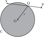
The previous examples have dealt with objects meeting head on, but in most cases, the objects that collide meet at an angle to each other. To deal with circles, a more general solution is needed, one that copes with circles of variable sizes colliding at variable angles. Fortunately, while this might seem to present difficulties, the fact is that you have already completed much of the work required to solve it.

As shown in Figure 8.4, the circle D(a, p) is approaching the circle C(o, r) with a relative velocity v. A larger circle of radius p + r has been drawn around O. At the moment of collision between the two circles, the line from A in the direction v enters the larger circle.

Figure 8.4. Two moving circles at an angle.

Given this information, it becomes possible to rewrite the pointCircleCollision() function so that it accommodates circles moving at an angle. What results is the circleCircleCollision() function:

function circleCircleCollision(cir1, cir2)
   set w to cir1.pos-cir2.pos
   set r to cir1.radius+cir2.radius
   set ww to dotProduct(w,w)
   if ww<r*r then return “embedded”
   set v to cir1.displacement-cir2.displacement
   set a to dotProduct(v,v)
   set b to dotProduct(w,v)
   set c to ww-r*r
   set root to b*b-a*c
   if root<0 then return “none”
   set t to (-b-sqrt(root))/a
   if t>1 or t<0 then return “none”
   return t
end function

In the preceding sections, you have considered circular objects colliding on the outside edge; however, as illustrated by Figure 8.5, you can also consider situations in which one circle bounces around inside a larger circle.

Figure 8.5. One circle inside another.

When one circle bounces around inside another, the situation is much like an external collision. However, in this case, at the moment of collision, the centers of the circles are separated by a distance, A, that is equal to the difference of the radii. Were the collision external, then they would be separated by the sum of the radii.

To create a function that addresses one circle bouncing around inside another, you can create a function that is almost identical to the circleCircleCollision() function. Since you are subtracting the radii rather than adding them, the circleCircleInnerCollision() function is no longer symmetrical. It tests whether circle 1 is inside circle 2, not the reverse. Also, notice that you now need to look for the larger root. As long as one circle is inside the other, the velocity vector always collides once in front of the circle and once behind.

function circleCircleInnerCollision(cir1, cir2)
   set w to cir1.pos-cir2.pos
   set r to cir2.radius-cir1.radius
   set ww to dotProduct(w,w)
   if ww>r*r then
      set rr to cir2.radius+cir2.radius
      if ww>rr*rr then return "embedded"
      return "outside"
   end if
   set v to cir1.displacement-cir2.displacement
   set a to dotProduct(v,v)
   set b to dotProduct(w,v)
   set c to ww-r*r
   set root to b*b-a*c
   set t to (-b+sqrt(root))/a
   if t>1 then return "none"
   return t
end function

Much can be said about the point at which a circle meets another object. First, you can quickly calculate the position of the point directly from the results of the functions discussed in the previous sections. Each of the functions returns a variable t that represents the fraction of the period of time that elapses before the objects collide. If you know the velocities of the objects (as you always do in these cases), then you can calculate shape.pos+shape.displacement * t to get the new position.

Second, you can determine the actual point of contact, although this will vary according to the situation. As shown in Figure 8.1, when a circle hits a wall, the point (P) of contact is along the perpendicular from the center of the circle to the wall. On the other hand, as shown in Figure 8.4, when two circles collide, the point of contact lies along the line joining the centers. This is in Figure 8.2. Whatever the position, the tangent of the circle at that point is perpendicular to the radius. This fact becomes important later on.

Although rectangles and squares have been examined in previous chapters, it is helpful at this point to review a few details. A rectangle is a two-dimensional shape with straight sides. Given this definition, it is often called a polygon. A rectangle has four vertices, making it a quadrilateral, and each of the four vertices is a right angle. Since both pairs of opposite sides of a rectangle are equal and parallel, it a parallelogram. For a rectangle ABCD, where the vertices are labeled clockwise, and , and is perpendicular to . A square is a special type of rectangle where the lengths AB and BC are equal and thus all the sides are equal.

The diagonals and meet at the center of the rectangle ABCD. In a square, these diagonals are perpendicular. The diagonal is equal to , and the diagonal is equal to . This is true for any parallelogram, which is why the rule for addition of vectors is often called the parallelogram rule.

You employ basic notation to define a rectangle. For example, you say that the rectangle R(u, v, w) is the rectangle centered on the point with position vector u whose sides are given by the perpendicular vectors 2v and 2w, where |v|>|w|. Although there are simpler approaches (see the previous note), you use this approach to defining a rectangle because it is simple and more symmetrical. As a side benefit, if you allow w to take any value, not just a vector perpendicular to v, you get a generic parallelogram, which means that many observations about rectangles generalize to arbitrary parallelograms.

Strictly speaking, the description just presented of a rectangle includes more information than you need. Since you can use the fact that two sides are perpendicular to determine the direction of the second side, you can just as well give only the vector for one side and the length (any positive scalar) for the other. With this approach, there is no potential for error. Every possible combination of three values yields a valid rectangle. Only in a degenerate case, where one side is zero, do you arrive at a straight line segment rather than a rectangle. As already mentioned, however, the first approach is simpler and more symmetrical.

With reference to the rectangle R(u, v, w), you can determine the vertices of R relatively effortlessly. They are u + (v + w), u + (v - w), u - (v + w), u - (v - w). Note that this ordering of the vertices is to be used in this chapter and those that follow. You also say that a rectangle is oriented in the direction of its long side, so R is oriented along the vector v.

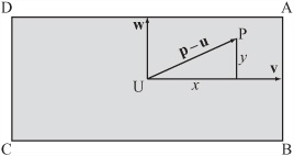
As illustrated by Figure 8.6, to develop a function that tests if a point P is inside the rectangle R, you find the components of the vector in the directions v and w. If the component in the direction v is shorter than |v|, and the component in the direction w is shorter than |w|, then P is inside ABCD.

Figure 8.6. Determining if a point is inside a rectangle.

The pointInsideRectangle() function applies this algorithm:

function pointInsideRectangle(pt, rectCenter, side1, side2)
   set vect to pt-rectCenter
   set c1 to abs(component(vect, side1))
   set c2 to abs(component(vect, side2))
   if c1 > magnitude(side1) then return false
   if c2 > magnitude(side2) then return false
   return true
end function

In the next chapter, you’ll look at another, more general method for testing if a point is inside a polygon. For now, notice that the pointInsideRectangle() function counts a point on the perimeter as “inside” the rectangle. If you don’t want to allow this, replace the > sign with >= signs.

To define a further function, you can also say that for any point P on the perimeter of R, if you take the vector , then either its component in the direction v has magnitude |v| or its component in the direction w has magnitude |w|. If both of these are true, then P is a vertex of R. Conversely, a point P is on the perimeter of the rectangle if this is true and also the point is “inside” R as defined by the definition previously given in this section of a rectangle. The pointOnRectangle() function applies these observations for any parallelogram:

function pointOnRectangle(pt, rectCenter, side1, side2)
   set vect to pt-rectCenter
   set c1 to abs(component(vect, side1))
   set c2 to abs(component(vect, side2))
   set s1 to magnitude(side1)
   set s2 to magnitude(side2)
   if c1 > s1 then return false
   if c2 > s2 then return false
   if c1=s1 or c2=s2 then return true
   // NB: for a safer test, use e.g. abs(c1-s1)<0.001
   return false
end function

As an extension of the previous section, consider the problem of detecting the collision between a stationary rectangle and a moving point. To solve this problem, you begin with the simplest case of a particle at P with velocity v passing through a plane that contains a rectangle R (u, a, b), as is illustrated in Figure 8.7.

Figure 8.7. A stationary rectangle and a moving point.

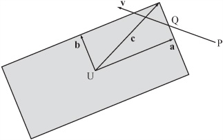
What you’re looking for is a point Q such that Q is on the trajectory of the particle, and Q is on the border of R. To solve this, you test for intersections with each of the four sides. At the first such intersection, the particle collides. The pointRectangleIntersection() function shows how such a function is implemented:

function pointRectangleIntersection(pt, rec)
   set c to rec.side1+rec.side2
   set t to 2 // start with a high value of t
   // then repeat over the four sides and look for the first collision
   repeat for v = rec.side1, rec.side2
      repeat for m = 1,-1
         set tl to intersectionV(pt.pos,
                                 pt.displacement,
                                 rect.pos-m * c,
                                 m * v * rec.axis*2)
         if tl = "none" then next repeat
         set t to min(t,t1[1])
      end repeat
   end repeat
   if t=2 then return "none"
   return t
end

The method used in the pointRectangleIntersection() function to loop through the four sides involves creating a vector. You create a vector c = a + b, which is the vector from the center of the R to one vertex. The implication of this construction is that -c is the vector to the opposite vertex. From the first of these vertices, two sides point in the direction -a and -b, and from the second, the other two sides point in the direction a and b.

The pointRectangleIntersection() function calls the intersectionV() function, which is a variation of the intersection() function used before. The intersectionV() function takes position-displacement information instead of four end points. It then returns a value of t for the intersection time if the two line segments intersect.

Because there is no smooth mathematical function describing all the points on a rectangle, many approaches to detecting collisions involving rectangles must be developed. Further, you often end up checking several possible options. This makes it necessary to be careful about potential problems at the vertices. With the pointRectangleIntersection() function example, a question arises concerning what happens if P lies somewhere along the line extended from one of the rectangle sides and moves parallel to that side. Does the function catch such a movement? Exercise 8.1 asks you to consider this type of problem.

The next problem beyond detection of collisions between particles and rectangles concerns collision between two rectangles. To start with the simplest case, as illustrated by Figure 8.8, a and b, consider a situation in which the rectangles are aligned along the same axis.

Figure 8.8. Two rectangles at the same angle (a) similar shapes and (b) differing shapes.

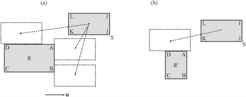
Figure 8.8 shows two rectangles, R and S, both of which are aligned along the axis u. In Figure 8.8a, depending on its velocity vector, rectangle S can collide with rectangle R in a number of different ways. However, they all boil down to six possibilities. In this example, at the point of collision, at least one of the three vertices J, K, L of S must be touching a side of R. The side that is touched is always either the side AB or the side AD of R.

Further, while K can be touching either AB or AD, J must be on AD (or both AB and AD) and L must be on AB (or both AB or AD). The other three possibilities arise from cases such as the one Figure 8.8b illustrates. Here the rectangle R’ is smaller along the colliding side than S, so at the point of collision none of the vertices of S is colliding with R’. However, the vertices of R’ are colliding with S, which means that you can perform a similar set of calculations the other way around. In the other direction, you need only check collisions for vertices B and D.

Since it is an adaptation of the pointRectangleCollision() function, which tests for intersection with all four sides, the rectangleRectangleCollisionStraight() function doesn’t take advantage of most of the optimizations just mentioned. You might want to see if you can come up with a faster implementation of the same test. One approach is to change the pointRectangleCollision() function as well. Still, here is one approach to dealing with collisions involving two rectangles:

function rectangleRectangleCollisionStraight(rec1, rec2)
   set t1 to rrVertexCollisionStraight(rec1, rec2)
   set t2 to rrVertexCollisionStraight(rec2, rec1)
   if t1="none" then return t2
   if t2="none" then return t1
   return min(t1,t2)
end function

Supporting the rectangleRectangleCollisionStraight() you make two calls to the rrVertexCollisionStraight() function, which as discussed previously, attends to detecting collisions:

function rrVertexCollisionStraight(rec1, rec2)
   set xvector to rec1.axis
   set yvector to normal(rec1)
   set r1 to rec1.side1*xvector
   set r2 to rec1.side2*yvector
   // calculate the points to test
   set points to pointsToCheck(r1.pos, r2.pos,
                               r1.displacement - r2.displacement)

   // now test each of these for intersection with the second rectangle
   set s1 to rec2.side1*xvector
   set s2 to rec2.side2*yvector
   set t to 2 // you're trying to find a value less than 1 for t
   repeat for each pt in points
      set t2 to pointRectangleIntersection(pt, rec)
      if t2="none" then next repeat
      set t to min(t, t2)
   end repeat
   if t=2 then return "none"
   return t
end function

As mentioned in the previous discussion, you check for position and displacement using the pointsToCheck() function:

function pointsToCheck(r1, r2, displacement)
   set points to an empty array
   set c1 to component(displacement, r1)
   set c2 to component(displacement, r2)
   if c1>0 then
      add r1+r2 to points
      add r1-r2 to points
   otherwise
      add -r1+r2 to points
      add -r1-r2 to points
  end if
  if c2>0 then
     if c1>0 then add -r1+r2 to points
     otherwise add r1+r2 to points
  otherwise
     if c1>0 then add -r1-r2 to points
     otherwise add r1-r2 to points
  end if
end function

Although developing three functions for detecting rectangular collisions at the same angle is somewhat complicated, it is not as bad as it looks. The complications arise only from having to check so many different cases. As points and rectangles, the same calculation can be performed with aligned parallelograms. With these, however, as differing from the approach used in the rrVertexCollisionStraight() function, you must specify the value of the yvector variable rather than calculating it from the normal given by the xvector variable.

A much simpler version of this process can be used if the rectangles are axis-aligned. Axis-aligned rectangles are aligned in the direction of the two basis vectors. This case is significantly easier to deal with, and you’ll return to it in a couple of chapters.

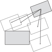
When rectangles are not aligned along the same axis, while you might think the problem gets a lot harder, it’s actually much the same. In fact, conceptually it is even easier than dealing with rectangles at the same angles. This is so because the point of contact will always be one of the eight vertices. As shown in Figure 8.9, you can narrow down the number of vertices to check to six, three from each rectangle.

Figure 8.9. Two rectangles at different angles.

As is shown in the rectangleRectangleAngledCollision() function, to work out which vertices to check, you can compare the displacement vector with the diagonals of the rectangles. Since they are all different, you give the values of the sides of the rectangle as vectors. This approach allows you to take advantage of work you have already completed:

function rectangleRectangleAngledCollision (rec1, rec2)
   set t1 to rrVertexCollisionAngled(rec1, rec2)
   set t2 to rrVertexCollisionAngled(rec2, rec1)
   if t1="none" then return t2
   if t2="none" then return t1
   return min(t1,t2)
end function

The rrVertexCollisionAngled() is called twice in the rectangleRectangleAngled Collision() function, and its responsibilities involve first arriving at the points to test and then testing for the points of interaction:

function rrVertexCollisionAngled(rec1, rec2)
  // calculate the points to test
   set axis to rec1.axis
   set points to pointsToCheck(rec1.side1* axis,
                               rec1.side2*normalVector(axis),
                               displacement)
   // now test each of these for intersection with the second rectangle
   set t to 2
   repeat for each pt in points
      set t2 to pointRectangleIntersection(pt, rec2)
      if t2="none" then next repeat
      set t to min(t, t2)
   end repeat
   return t
end function

As the code in this and the previous section illustrates, no significant differences arise between calculations of aligned and non-aligned rectangles. One of the only points of concern is with axis-aligned boxes, which is the topic of a subsequent section.

A major difference between working with smooth objects like circles and polygons, as with rectangles, is in the point of contact. When two smooth objects collide, there is always a precise normal at the point of contact, and this defines the collision precisely. With polygons, this is no longer the case. Either you have a collision between two edges of the polygon, as in Figure 8.8, or between an edge and a vertex, as in Figure 8.9.

If a collision occurs between two edges, detecting the collision involves recognizing that the normal is simply the normal of the meeting edge. However, a vertex doesn’t have a normal. When a vertex and edge of a polygon meet, you might expect almost anything to happen. Actually, it’s not that bad. When the vertex meets an edge, there is always at least one well-defined normal.

Otherwise, things are reasonably straightforward. It is simple to adapt the given functions to return the point of contact of the rectangles and other useful information.

Likewise, detecting collisions between a rectangle and a wall is almost identical to detecting collisions between two edges. A wall is a rectangle that is much bigger than the rectangle colliding with it. Since you do not need to test for collisions between the wall vertices and the rectangle vertices, you cut the problem in half. You can also perform collisions with a line segment. A line segment is essentially a rectangle with one pair of sides having zero length.

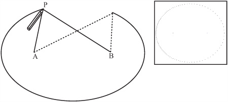
An ellipse is to a circle what a rectangle is to a square. It is a circle stretched in one direction. One way to imagine drawing an ellipse is to take a length of string and attach it to two drawing pins on a piece of paper at points A and B. As shown in Figure 8.10, putting the tip of the pencil to the paper and pulling the pencil around the inside of this string results in an ellipse. This shape is distinguished by the fact that for any point P on the perimeter, the sum of the distances AP and BP is constant. The length of the string does not change.

Figure 8.10. Drawing an ellipse. (Inset: a computer-generated ellipse.)

The two points A and B are called the foci of the ellipse, and the length AP + BP is the internal diameter. Notice that if A and B are the same point, then the ellipse becomes a circle, and the internal diameter is equal to the diameter of the circle. “Internal diameter” is not a formal term used with ellipses, but it conveys the idea that an ellipse differs from a circle by the addition of these two lines.

Developing a function to draw an ellipse can take any number of paths. The drawEllipseByFoci() function represents one approach. It generates an ellipse given the foci and internal diameter. Likewise, note that a function discussed in Chapter 5, the angleBetween() function, is used in its implementation.

function drawEllipseByFoci(focus1, focus2, diameter)
   set resolution to 100
   // increase this number to draw a more detailed ellipse
   set angle to 2*pi/resolution
   set .angleOfAxis to angleBetween(focus2-focus1, array(1,0)
   if angleOfAxis="error" then set angleOfAxis to 0
   set d to magnitude(focus1-focus2)
   set tp to diameter*diameter-d*d
   repeat for i =1 to resolution
      set a to angle*i // the angle made at focus1 with the major axis
      set k to tp/(2*(diameter-d*cos(a)))
      set ha to a+angleOfAxis
      set p to k*array(cos(ha),sin(ha))
      draw point p
   end repeat
end function

The drawEllipseByFoci() function does not provide a purely mathematical approach to drawing an ellipse, but you might want to see if you can use a mathematical approach. To accomplish this, the key is to use the cosine rule on the triangle PAB. The drawback to a purely mathematical approach, however, is that it draws more points around one focus than the other. On the right of Figure 8.10 is an ellipse drawn by using a mathematical approach. The dots on the left half of the perimeter are more dense than those on the right.

Rather than the approach presented in the previous section, you can describe an ellipse using coordinate values. To understand how this is so, remember that every point on a circle centered on (0,0) with radius r has coordinates for some . A similar description holds true of an ellipse. The shape traced by the points with coordinates is an ellipse with internal diameter and foci at and . Assuming that a > b, the lengths a and b are called the semi-major and semi-minor axes, respectively.

However, this approach draws only an ellipse aligned along the x-axis. In this case, you say that the ellipse is aligned along the vector of its major axis. The major axis is the vector between the two foci. If you want this ellipse to be rotated so that its axes are not aligned with the major axis, drawing the ellipse becomes complicated. You must adjust each point by rotating it by a constant angle around the center of the ellipse. With the assistance of a function that adjusts points, the drawEllipsesByAxes() function plots an ellipse using coordinate values:

function drawEllipseByAxes(center, a, b, alpha)
   set resolution to 100 // increase to draw more accurately
   set ang to 2*pi/resolution
   repeat for i =1 to resolution
      set angle to ang*i
      set p to rotateVector(array(a*cos(angle), b*sin(angle), alpha)
      draw point center+p
   end repeat
end function

The rotateVector() function takes care of the work of rotating the ellipse. In addition to making the code easier to understand, refactoring the code into two functions makes it possible to use the rotateVector() function in other contexts discussed later on.

function rotateVector(v, alpha)
   set x to v[1]
   set y to v[2]
   set l to sqrt(x*x + y*y)
   set x1 to l*cos(alpha-atan(y,x))
   set y1 to l*sin(alpha-atan(y,x))
   return array(x1,y1)
end function

Although the two approaches to plotting an ellipse, shown in the previous two sections, are largely equivalent, in different circumstances, each has certain advantages. Still, the most useful is the second, for it appeals to the idea of an ellipse as a stretched circle. To state this precisely, any ellipse centered on the origin can be created from a unit circle. To do so, first scale the space by a factor of a in one direction and a factor of b in the other. Then rotate the ellipse to point in the correct direction. You can describe this with a standard transformation matrix T, made up of a scale followed by a rotation. After you’ve done this, you can translate the ellipse to the correct position. You use the notation E(c, T) to describe such an ellipse. The drawEllipseFromMatrix() function warps the previously discussed drawEllipseByAxes () function to accomplish this task:

function drawEllipseFromMatrix(pos, mat)
   set v to mat.column
   set n to mat.column
   drawEllipseByAxes(magnitude(v), magnitude(n), atan(v[1],v[2]))
end function

One common term used with ellipses is the value , known as the eccentricity of the ellipse. The higher the eccentricity, the more “pointy” an ellipse becomes. An eccentricity of 1 gives a circle, while an eccentricity of infinity gives a straight line.

A final useful fact about an ellipse is that the tangent to the curve at P makes the same angle with each of the lines AP and BP. If you have an elliptical pool table with a ball at one focus and a pocket at the other, hitting the ball in any direction results in the ball going in the pocket. On an ellipse aligned along the x-axis, at the point , the tangent lies along the vector .

Suppose that the particle at P is moving with velocity v in space occupied by the ellipse E(c, T). A question that arises is whether the point enters the ellipse. To answer this question, consider first translating to the ellipse’s frame of reference. You accomplish this by subtracting c. Having done this, you end up with a vector equation:

If you invert the matrix T using the methods discussed in Chapter 5, you end up with this equation:

Since u is a unit vector, you know that its dot product with itself must be 1. As a result, you reach this equation:

This version of the equation might appear familiar. You are looking at the intersection of a particle with a unit circle, a problem dealt with earlier in this chapter.

As an approach to developing a function to detect collisions of ellipses and particles, it is helpful to think about it geometrically. Consider Figure 8.11. In (a) you have the generalized ellipse. In (b) you have rotated the ellipse to a new frame of reference, with the axes aligned with the basis. In a final step, not shown in the figure, you can compress the space down to turn the ellipse into a circle. Although everything is moving about the displacement vector accordingly, the relative distances along the lines don’t change even if the absolute length does. Here you can really see the power of the relativity principle.

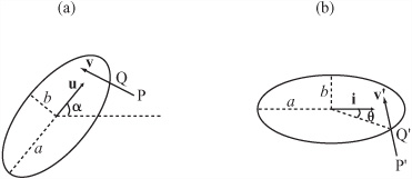
Figure 8.11. A stationary ellipse and a moving point (a) in the plane and (b) rotated to the ellipse’s frame of refer-

The particleEllipseCollision() function implements an algorithm based on the previous discussion. Its arguments are the ellipse and the point, and as with other functions examined in this chapter, it draws from functions introduced in Chapter 5.

function particleEllipseCollision(pt, ell)
   set t to ell.transformationMatrix
   set inv to inverseMatrix(t)
   set p to pt.pos-ell.pos
   set w to matrixMultiply(inv,p)
   set ww to dotProduct(w,w)
   if ww<1 then return "inside"
   set v to matrixMultiply(inv,pt.displacement-ell.displacement)
   set a to dotProduct(v,v)
   set b to dotProduct(w,v)
   set c to ww-1
   set root to b*b-a*c
   if root<0 then return "none"
   set t to (-b-sqrt(root))/a
   if t>1 or t<0 then return "none"
   return t
end function

If two ellipses that happen to be aligned in the same direction meet head on, their collision is an easy analogue of the circular case. Such luxuries are sadly not to be had in the more general case where two ellipses E(p,S) and F(q,T) meet with arbitrary velocities. As in previous examples, you can apply the relativity principle to bring the problem down to a simpler case, a stationary unit circle meeting the ellipse F’(q–p, S^-1 T). Unfortunately, this time the principle does not help you as much as it might. Ultimately, you end up with a highly complicated pair of nonlinear simultaneous equations that are not easily untangled.

There is one additional trick that can help you. You can use the fact that at the point of collision, the normals on the two surfaces are parallel. This is the key to the whole issue, but you don’t yet have the tools and vocabulary to deal with it. For this reason, you’ll return to the question in Chapter 19.

To determine the point of contact of an ellipse with its partner in collision, you can use the same approach you used with circles, but a bit more caution is needed. From the value of t in each of the functions dealt with previously, it is trivial to calculate the collision position of the moving bodies in your simulation. But to determine exactly where on the shapes they collide, you must transform back into the correct reference frame. This requires you to find the point of contact in the transformed frame, and then transform this point again with T.

It’s all very well to have these nice neat calculations for objects of the same kind, but what happens if you want to deal with more natural situations? Fortunately, it turns out that calculations with similar shapes can be easily adapted to such mixed events. In Figure 8.12 you can see a circle C(p,r) heading toward the rectangle R(u, a, b) with velocity v. Notice how, as v varies, the situation falls into three possible forms:

Figure 8.12. A collision between a circle and a rectangle.

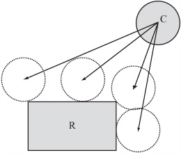
In the first case, you can calculate the point of contact by considering the vertices of R and checking for intersection with C using the pointCircleCollision() function. In the second, you can think of the edge of R as a line segment or a wall, and use the circleWallCollision() function to handle it. Alternatively, you can expand the rectangle by the circle’s radius in all directions and then apply the pointRectangleCollision() function. In both cases, you can work out in advance which of the vertices or edges are potentially involved in the collision just as you did with rectangle-rectangle collision. In the third case, no function developed so far helps or for that matter is needed.

Collisions between circles and rectangles are much the same as collisions between rectangles and rectangles in terms of the point of contact. Whether the collision is with an edge or a vertex, the normal is always the normal to the circle at that point. However, when the collisions involves an edge, it’s easier to calculate the normal to the edge.

Write a function named pointParallelogramCollision(). As parameters, use pt, displacement, parrPos, side1, side2. As a model, use the pointRectangleCollision() function discussed in this chapter. Your function should return a value between 0 and 1 or the string “no intersection”.

To write this function, take advantage of the fact that a parallelogram can be transformed into a rectangle by applying a skew transformation to the plane. You can do this within a complete function or call the pointRectangleCollision() function.

Write functions named rectangleRectangleInnerCollision(), circleRectangle InnerCollision() and rectangleCircleInnerCollision() with appropriate parameters in each case to test for collisions inside shapes.

As with the case of a circle colliding with a circle, these inner collisions are very similar to the external ones covered in this chapter, but they each have subtle complications of their own. Use the code in the chapter to help you where possible.