
This is a second chapter on fundamentals. In this chapter, the central concern is the principles of algebra, a branch of mathematics that deals with variables. Consideration is first given to the basic principles of algebra. After that, specific techniques are explored. The explorations include methods for using graphs to visualize equations and functions.
This section reviews a number of terms used in algebra. The terminology of algebra is extensive and essential for all areas of mathematics that are built on it. Given a beginning with terminology, the stage is then set for discussions of equations and other topics.
You represent two basic types of value in algebra. One is called a constant. The other is called a variable. Both of these values are usually represented as letters. Most people are familiar with them as the letters a, b, c, or x, y, z. A constant does not change. A variable does. Various names are applied to constants and variables depending on how they are used. The following list reviews the primary uses of variables and constants.
Constant. A constant is a value that does not change. Examples are the constants e and ϕ. Likewise, values as represented by such symbols “1” and “2” are also constants. A constant can be an arbitrarily assigned value, as when you temporarily define the letter A to stand for the expression
 .
.Parameter. A parameter is a value that defines a family of similar mathematical objects. For example, in the linear equation y = m × x + c, the parameters m and c are used in all examples of this equation. The values substituted for m and c always convey the same type of information. You know what the value stands for.
Unknown. An unknown is a token that represents a value that you do not know. For example, if you know that x is a particular number, and that x + 3 = 4, then you can calculate the (unknown) value of x.
Variable. A variable represents something that can be of any value. This is like an argument passed to a function in the computer. For example, you can write a function that calculates the cube root of some number n, and n in this function is a variable.
You’ll notice that these terms are a little fuzzy. After all, in the equation x + 3 = 4, you can call x an unknown. On the other hand, it is also a variable, for you can substitute a value into it (1). If you consider the equation at length, you also see that the value that you substitute for x is always the same, so x is a constant.
The easiest way to think of these terms is as a hierarchy of variability. If you have an expression with a lot of letters, say u + a × t, you can decide that one or more of these are “fixed,” and the others are “variable.” The fixed terms might be called parameters. For a particular set of parameters, you have a particular behavior for the variable terms. Then you might fix one of the parameters even more strongly and call it a constant. Each choice of a constant gives you a family of families. Finally, you can vary the constant to give you a family of families of families!
Variables and constants are used in similar ways by mathematicians and programmers. There is one difference that stands out, however. Programmers are encouraged to create mnemonically significant variable and constant names. For example, rather than naming a variable in a program x, a programmer is encouraged to use a name such as numOfPlayers or accountNumber. Likewise, due to language conventions, programming languages might represent the Greek letter π with the characters PI. Constants, generally, are represented by words consisting of capital letters.
A mathematical combination of variables or constants is called an expression. For example, (a × x) + (x2 × 4) + 3 is an expression using the variables a and x, and the constants 3 and 4. Another constant also appears. This is the 2 used as an exponent, which is shorthand for the expression x × x.
Note
As in manual evaluations, most compilers evaluate mathematical expressions in a standard order. First, expressions in parentheses are evaluated recursively. Next, other operators are evaluated sequentially: parentheses, division and multiplication, subtraction and addition. Thus the expression 1 + (2 × 3 – 4) × (–5 + 6) evaluates to 1 + 2 × 1, or 3. Expressions used as the numerators or denominators of fractions are considered to be in parentheses.
A term is any subexpression of the main expression that does not contain additions or subtractions. It is convenient to group expressions into terms. With (a × x) +(x2 × 4) + 3, if you consider x to be a variable and a to be a constant, then there are three terms, a × x, x2 × 4, and 3. A term can contain any number of variables multiplied by a constant, which is called the coefficient. In the term x2 × 4, 4 is the coefficient of x2.
Terms can be classified according to the exponents of the variables within them. The terms 3 × x2 and –2 × x2 are considered like terms because they both have the same exponent of the variable x, namely 2. On the other hand, 3 × x2 and 3 × x are not like terms, because they contain different powers of x. Two terms are alike if they only differ by their coefficient.
To extend the discussion, consider the expressions 2x and p(1 + q). In both expressions, two or more values are written next to one another. Such a construction indicates that a multiplication is to be performed. As a general rule, a coefficient is always written before the variables (2x, not x2), and terms outside parentheses are written first p(1 + q), not (1 + q)p. A term is usually written as a single string without multiplication signs, so the expression a × x + x2 × 4 + 3 is written as ax + 4x2 + 3. This allows you to easily group terms according to the exponents of their variables. For example, you see the x term, the x2 term, and then the constant.
A function is a map that takes values from one set, called the domain of the function, and transforms them into values from the same or another set, called the range of the function. Consider a situation in which rational numbers are transformed into integers. Functions in mathematics are usually represented as a single letter followed by open and close parentheses between which the parameter of the function is represented. For instance, the equation y = f(x) indicates that the value x in the domain is mapped to the value y in the range. Functions are usually read as “f of x.” The value of the range is a function of the value of the domain. If you have a function f(x), then you refer to the value f(3) as the result of substituting 3 for x in the function. The result of substituting 3 for x in the function x → x(x + 2) is the value 3 × (3 + 2) = 3 × 5 = 15. (The arrow is a logical symbol for “x maps to.”)
What applies to math also applies to programming. Consider the floor() function, introduced in Chapter 1. When you use this function, you feed it a number that is not an integer (3.45, for example). It then returns an integer (3). You can also have Boolean functions, which map their input to just two values, 0 and 1. As an example, one common Boolean function is named isPrime(). This function returns 1 if the input is a prime number and 0 otherwise. In typed computer languages, you generally need to specify in advance both the type of the input value of a function and the type of the output value. For example, you designate that the function requires an integer argument as input and returns a double (a floating-point value). This requirement formalizes the fundamental nature of functions, which requires that they draw from a specific domain and translate to a specific range.
Many mathematical functions have their own symbols, and these symbols are represented in program functions. The ![]() symbol represents the
symbol represents the sqrt() function. Some mathematical functions directly correspond to program functions. Among these are sin(), cos(), and tan(). In other instances, the correspondence is not so clear. Consider the function x2 + 2. This function might be formally expressed like this:
square Plus Two(x: R→R) =x2 + 2
The R → R part of this formulation is required in a formal definition of a function. It is not necessary to include it in this context, however. In this case, all it means is that both the input and output of the function are real numbers.
Note
The second R could be replaced with a >R+, signifying the set of positive real numbers, since you know that the output of the function is always positive. Even more accurately, it could be said that the range of the function is the set [2,∞]. This is a common notation for the set of real numbers from 2 to infinity. In this case, the function is shown to map to the whole of the range.
If you have a function f(x) and there are no two distinct input values a and b in its domain such that f(a) = f(b), then you call the function one-to-one. For such functions, there is also an inverse function, sometimes expressed as f’. With an inverse function, for every a in the function’s complete domain, f’(f(a)) = a. For example, the cube function, x → x3 is one-to-one. On the other hand, the square function, x → x2 is only one-to-one when considered over the domain of positive real numbers (a partial or limited domain). A function for which values in the domain map to the same value in the range is called many-to-one.
Functions are multivalued when there is at least one value in the range that can map to more than one value in the domain. Among these is the mathematical square root function. With this function, both 1 and –1 are square roots of 1. Multivalued functions are usually the inverses of many-to-one functions, as in the case of the square root function. Strictly speaking, these are not functions at all, but it is useful to refer to them as functions. As a further point, it is impossible for self-contained functions programmed using standard programming languages to be multivalued. For example, the sqrt() function is a regular one-to-one function from R– to R+, and it always returns a positive square root.
A polynomial is a particular kind of function of the form ![]() anxn where the values a0, a1, a2,... are all real numbers. Polynomials are distinguished according to degree. The function x → 2x + 1 is a polynomial. It is called a linear or first-degree polynomial because the highest power of x is 1. The function x → 2 – x + 3x2 is a quadratic or second-degree polynomial because the highest power of x is 2. It is also possible to have polynomials in more than one variable, such as x → x2 + 2xy + y2.
anxn where the values a0, a1, a2,... are all real numbers. Polynomials are distinguished according to degree. The function x → 2x + 1 is a polynomial. It is called a linear or first-degree polynomial because the highest power of x is 1. The function x → 2 – x + 3x2 is a quadratic or second-degree polynomial because the highest power of x is 2. It is also possible to have polynomials in more than one variable, such as x → x2 + 2xy + y2.
Note
Discussion of functions has been formalized so far in this section, but a degree of informality makes things easier to communicate. From now on, such expressions as x2 + 1 will be referred to as functions. This removes the need for expressing functions using the mapping notation of mathematics: X→X2+1
An equation is like a mathematical sentence. It states that one expression is equal to another. Consider 1 = 1. This is a simple and rather obvious equation, as is 2 + 2 = 4. In most contexts, the term equation refers to a sentence that includes a variable, such as x + 2 = 5. This is a sentence that tells you a fact about the unknown x. In this case, it tells you enough about it that if you know that the equation is true, you can deduce what the value of x must be, namely, x = 3. The process of deduction is the main focus of elementary algebra.
It is important to distinguish between a function, an expression, and an equation. A function is like a phrase with blanks in it. It might read, “The --- with tall ---’s.” An expression goes a step farther. It fills in the blanks with dummy variables: “The nnn with tall mmm’s.” An equation then tells you something about this expression by relating it to another. “The nnn with tall mmm’s is a qqq.”
Of the three activities, only an equation can be true or false. In this case, you don’t know whether it is true or not because you don’t know what an nnn, an mmm, or a qqq are. But if the sentence were “an nnn is an nnn,” then you could know it is true, whatever an nnn might turn out to be. Such an equation is called a tautology. For example, x + 2 = x + 3 – 1 is a tautology because it is true no matter what the value of x is. The equation x + 1 = 2 is not a tautology, however. If x = 1, then the equation is true. If x is any other value, then it is false. The same happens in a program. If you are working with a variable x, and you have the line, if x + 2 = 3, then the program executes the next line if and only if x = 1—that is, if the equation is true. Reversing the reasoning, if you know the equation is true, then you know the value of x must be 1.
A formula is an equation with more than one variable, and it defines one variable in terms of others. For example, v = u + at is a formula that defines the value v in terms of the variables u, a and t. However, since formulas and equations can be treated identically, this is just a terminological distinction. Formulas are most often used to express relationships between physical values, such as distance = speed × time.
An inequality is like an equation, but it tells you something other than that the two equations are equal. The types of inequalities vary fairly extensively. An inequality might say that one expression is less than the other. Consider, for example, x + 1 < x + 2. This happens to be a tautological inequality, for it always true, no matter what the value of x. An inequality might also say that one expression is greater than another. Consider, for example x + 1 > y. This is an inequality that might or might not be true, depending on the values of x and y. On the other hand, an inequality might simply assert that two expressions are not the same. In a computer language, you might write x != y or x <> y. Mathematically, you usually write x ≠ y.
Other symbols for inequalities are compounded or more abstract. Consider ≤ and ≥, representing “less than or equal to” and “greater than or equal to.” Still another symbol, not asserting inequality but instead a limited form of equality, is ≈, meaning “approximately equal to.” There is also the congruency symbol ≡. The latter two are not generally referred to as inequalities, but neutrally as statements.
Algebra allows you to make deductions about unknown quantities by manipulating them as symbols rather than calculating with them directly. This section reviews the primary techniques involved in algebraic manipulations.
An equation is said to be like a set of scales. If you know that a pair of scales balances, then you know that if you add or take away the same amount from each side of the scales, the scales will still balance. The same is true of an equation. The two expressions on each side of the equals sign are equal by definition. If you add the same value to both sides, they will still be equal. In fact, if you apply any non-multivalued function to both sides of an equation, the equation remains true.
Why specify that the function must not be multivalued? Imagine that you have the equation a2 = b2. It is tempting to take the square root of both sides of the equation, yielding a = b, but this is not necessarily true. It is not true because if a = 2 and b = –2, then the first equation is true but the second is not. This is because the function x ![]() is multivalued. Two distinct values in its domain can map to the same value in the range. All you can say with safety is that a = ±b, where the ± symbol means “plus or minus.”
is multivalued. Two distinct values in its domain can map to the same value in the range. All you can say with safety is that a = ±b, where the ± symbol means “plus or minus.”
The process of solving an equation in an unknown involves performing operations on both sides of the equation to find the value of the unknown. The most general equation is something like f(x) = g(x) for some functions f and g. If you subtract g(x) from both sides of the equation, you have f(x) – g(x) = 0. This can be as a new function q(x), where q(x) = f(x) – g(x). Generally, then, in its simplest terms, solving an equation is trying to find the inverse of the function q at 0.
Consider a less theoretical example. Suppose the equation is 2x + 3 = 7. Here, the left-hand side of the equation has two terms. One term contains x. The other provides a constant. To solve the equation, you can begin by subtracting the constant from both sides:

Now you have an equation with one term on each side. On the left-hand side is a multiple 2 of x. On the right-hand side is a constant, 4. Now, to isolate the value of x, divide both sides by 2:
Using this process, you find the value of x, which is 2. If you check the work, you find that 2 × 2 + 3 is indeed equal to 7.
As was emphasized previously, you can think of 2 × 2 + 3 differently, in terms of functions. If you do this, you have a function x→2x+3 which presents a good starting place for exploring inversion. Since the function multiplies by 2 and then adds 3, the inverse is a process of subtracting 3 and then dividing by 2. This amounts to the reverse steps in the reverse order. The inverse function is x→(x–3)/2. If you apply this function to both sides of the equation, the left-hand side maps to x (by the construction of the inverse function), and the right-hand side maps to (7 – 3)/2 = 4/2 = 2. This activity is the same as what was done previously, but the reasoning behind it is a little different.
It isn’t always so easy to solve an equation through inversion. Consider the equation ![]() . You have a bit of work to do before you can isolate the value of x. To do so, you must resort to simplification. To simplify an equation (or function), you reorganize it so that it is in successively simpler forms. In the end, you reach the simplest form. What constitutes the simplest form depends on the circumstances, but there are a few processes that you can apply regardless of circumstances. Here is a short list:
. You have a bit of work to do before you can isolate the value of x. To do so, you must resort to simplification. To simplify an equation (or function), you reorganize it so that it is in successively simpler forms. In the end, you reach the simplest form. What constitutes the simplest form depends on the circumstances, but there are a few processes that you can apply regardless of circumstances. Here is a short list:
Group like terms. Like terms are terms that contain the same combination of variables, differing only by the coefficient. With 2x + 3x = 5x, two terms 2x and 3x are like terms and so can be combined into one.
Cross-multiply. Drawing from the discussion in Chapter 2, the expression

can be simplified to

This might seem involved, but if you substitute 4 for x, it is the same process as in

Remove fractions. If you have a fraction on one side of the equation, to remove the fraction, multiply both sides of the equation by the denominator. Using this approach,
 becomes x = 2 (x + 1).
Multiply out parentheses. If you have a product of one element with an expression in parentheses, multiply the outside element by each element inside the expression to create an expression with no parentheses. Here are a few examples of this:
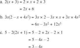
The third example (c) in the previous list proves troublesome due to the minus sign in the first expression of the equation. Items within the parentheses are multiplied by –2. When multiplying values within parentheses by a negative number, the negative number applies to all values inside the parentheses. To explore a different view of this topic, suppose that the original expression had been written as 5 + (–2) × (2x + 1). Comparing this version of the equation with the original allows you to see the effect of the negative sign.
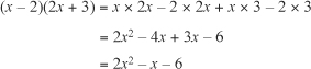
Beyond negatives, you can also multiply together the values contained by parentheses. One approach to such a problem is to split it into two steps. Here is an example of how to proceed:
To extend the discussion, if you encounter an expression that is common, you might be able to transform the equation into another form by defining a new variable. While this is an obscure technique, it is useful in complicated circumstances. For example, suppose you want to solve the equation 4x4 – 9 = 0. Notice that 4x4 = (2x2)2. To simplify the expression, you can substitute a variable, p, defining it as p = 2x. Since 4x4 = p2, you have p2 – 9 = 0, or p2 = 9. Since the square root of 9 is 3, p2 = ±9.
Now to find x, you simply substitute back into the definition. Accordingly, since p = 2x2, 2x2 = ±3. Likewise, since 2x2 must be positive, you can ignore the negative square root of p. As a result, 2x2 = 3, so ![]() . As already mentioned, this is an exceptional and difficult technique you encounter only on occasion. It is used, for example, later in this chapter with equations involving cubed values.
. As already mentioned, this is an exceptional and difficult technique you encounter only on occasion. It is used, for example, later in this chapter with equations involving cubed values.
Look again at the equation with which this section began. It provides an occasion for applying some of the notions developed in the previous sections.
To solve this equation, begin by simplifying the denominator. Toward this end, multiply out the parentheses:
Now combine like terms in the denominator:
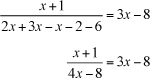
To clean up the fraction, multiply both sides of the equation by the denominator. This gives you:
Now multiply out the parentheses on the right-hand side to get:

Finally, bring the terms from the left-hand side to the right-hand side and simplify again:

In the last line, the expressions have been switched (putting the 0 on the right). This is a traditional form of presenting an equation. When you have an equation with a constant on one side, you put the constant on the right. The practice corresponds to the convention in English of putting a proper noun before the verb in a sentence that contains a copulative verb. For example, speakers of English say, “Patch is a dog,” rather than “a dog is Patch.”
Another simplification technique goes in almost the opposite direction of multiplying out the values in parentheses. Rather than multiplying out the values in parentheses, it simplifies the expression by finding common factors. The approach is the same as used in Chapter 2 when the gcd() function was applied to denominators to simplify addition of fractions. When working with plain numbers, this is called factorization, or more commonly, factoring.
In general, it’s best to leave factoring until you have already gone through the simplification process discussed in the previous section, joining all the like terms together and eliminating fractions with variables in the denominator. When working with an equation, it also a good idea to move all the terms over to one side, giving you an equation of the form f(x) = 0. Factoring, strictly speaking, is an operation performed on functions rather than equations.
Having expressed the equation as a function, you try to find any common factors between the terms. For example, in the expression 6x2 – 15x + 9, all the terms have a factor of 3. You can take out the factor of 3, making it a separate term, to get 3(2x2 – 5x + 3).
Another example is x2–4x. Here, both terms have a factor of x. As before, you factor the expression on the left-hand side of the equation by turning it into a product of the factor x. To express this change, you use parentheses. First you write x, then, in parentheses, you write the value of x–4. This gives you x(x–4).
Note
If this isn’t clear, try multiplying together the terms inside and outside the parentheses to see what you end up with. It is the same process as in the previous case, but with a factor of x instead of the number 3.
You can use the factored version of a function to make it easier to solve equations. If you have 3(2x2 – 5x + 3) = 0, for example, you can divide both sides by 3 to get a simpler equation, 2x2 – 5x + 3 = 0. And if you have x(x – 4) = 0, then you have two unknown numbers (x and x – 4) whose product is zero. If the product of two numbers is zero, you know that either one or the other number must be zero. This means that you end up with either x = 0 or x – 4 = 0. The value of x, then, is either 0 or 4.
Given the preliminary discussion, here are some specific examples of factoring:
12x3 – 8x2 has a common factor of 4x2, because 4 is a factor of both 12 and 8. x2 is a factor of both itself and x3. This makes it possible to isolate this factor, resulting in the expression 4x2(3x + 2).
–2x – 3x2 has a common factor of –x. Since a negative number divided by a negative number is positive, factoring this expression you arrive at –x(2 + 3x).
2xy2z + 4x2yz has a common factor of 2xyz. Factoring, the outcome is 2xyz(y + 2x).
 has a common factor of
  . Think of this as a two-stage process. The first involves simplification:
  . After further factoring, you end up with
In addition to factors that are simple terms, whole expressions can be taken as factors. For example, in the expression x(x + 1) + 3(x + 1), the expression (x + 1) is a common factor, so the expression can be factored to (x + 1)(x + 3).
Consider what happens if you multiply out the terms in parentheses of (x + 1)(x + 3) and then join the like terms. This results in x2 + 4x + 3. To factor this expression, given that you just performed the multiplication that created it, you can reverse the process and fairly easily reach its factored form. It is clear, however, that expressions such as x2 + 4 x + 3 are not as easily factored as expressions like x(x + 1) + 3(x +1).
The expression x2 + 4x + 3 is a quadratic expression. A quadratic is any expression of the form ax2 + bx + c. If a quadratic expression can be factored, it takes the form (px + n)(qx + m).
Note
As a matter of review, in such generalized terms as ax2 + bx + c and (px + n)(qx + m), a, b, p and q are place holders for coefficients. Unless its value is greater than 1, the coefficient is not usually represented by a literal expression. For example, you usually do not write 1x2 + 1x + 2 (where c, a constant, is equal to 2).
To develop a general pattern for simplifying quadratic equations, you can equate the two expressions using the equation ax2 + bx + c = (px + n)(qx + m).
If you multiply out the expression on the right-hand side and then combine terms, the equation assumes the following form:
This is an equation in which x is a variable, while a, b and c are parameters. For any possible value of x, given particular values of a, b and c, the equation is supposed to be true for any possible value of x. If this is to be so, each of the terms in x must match. As a result, if you assume that p= 1, you can reason as follows:

Consider a case in which a= 1. The general form of the quadratic becomes x2 + bx + c. As a result, moving to the corresponding expression, n + m = b, and nm = c. Further, n and m are two numbers whose product is c and whose sum is b.
How can you find these numbers? One approach is to use inspection. Here are a few examples:
x2 + 4x + 3. Since b = 4 and c = 3, you need numbers whose product is 3 and whose sum is 4. These numbers are 1 and 3. So the expression factors to (x + 1)(x + 3). (This is the same as the result shown previously.)
x2 + 3x – 4. Since b = 3 and c = –4, you need numbers whose product is –4 and whose sum is 3. The numbers 4 and –1 meet this description. So the expression factors to (x + 4)(x – 1).
x2 –5x + 6. Since b = – 5 and c = 6, you require numbers whose product is 6 and whose sum is –5. The –2 and –3 meet this description. The expression factors to (x – 2)(x – 3).
x2 –5x – 6. Since b = – 5 and c = –6, you need numbers whose product is –6 and whose sum is –5. These numbers are –6 and 1. The expression factors to (x – 6)(x + 1).
Notice that the numbers you are looking for vary according to the sign of the numbers b and c. In the last two examples, the absolute values of b and c are the same, but because the sign of c is different, the answer is changed significantly.
Can you always find two numbers, n and m, that satisfy this requirement? The answer is no. For example, if b = 1 and c = 1, then no pair of numbers whose sum and product are both 1 exists. As a general rule, you can only factor a quadratic expression as long as b2 ≥ 4ac. This expression is called the discriminant. Why this is so is discussed shortly.
Given the quadratic form ax2 + bx + c, what if a is not equal to 1? When this is so, you can reason things as follows:
In this case, you are looking for two values, am and n, whose sum is b and whose product is ac. While the technique used to factor remains much the same, after you have found am, you need to divide it by a to find m.
As an example, consider an equation examined earlier: 12x2 – 57x + 63 = 0. To factor this equation, start by dividing the whole equation by a common factor, 3. This division results in 4x2 – 19x + 21. For this equation, b = –19, and ac = 4 × 21 = 84. Consequently, you are looking for two numbers whose product is 84 and whose sum is –19. These numbers are –7 and –12. You can choose either one of these to be n and am. Since a = 4, however, and 4 is a factor of 12, it makes sense to choose n = –7, and m = –3. This way, it is not necessary to use fractions.
Given these preliminaries, you arrive at 4x2 – 19x + 21 = (4x – 7)(x – 3). Working from the notion that the product must be zero, you also know that either x – 3 = 0 or 4x – 7 = 0. Working these out, you find that either x = 3 or x = 7/4. To test, substitute either of these values into the original equation and see if it evaluates correctly to 0.
The most prevalent way that most people learn to solve quadratic equations involves using the quadratic formula, which reads, ![]() . To work with this formula, notice that if b2 < 4ac, then the value under the square root sign is negative. There is no real number solution for x in these circumstances. If b2 > 4ac you arrive at two values for x, one using the positive square root, the other using the negative. If b2 = 4ac, then the quadratic equation is an exact square, and there is only one solution for x. This occurs in an equation such as x2 – 6x + 9 = 0, which factors to (x – 3)(x – 3), or (x – 3)2.
. To work with this formula, notice that if b2 < 4ac, then the value under the square root sign is negative. There is no real number solution for x in these circumstances. If b2 > 4ac you arrive at two values for x, one using the positive square root, the other using the negative. If b2 = 4ac, then the quadratic equation is an exact square, and there is only one solution for x. This occurs in an equation such as x2 – 6x + 9 = 0, which factors to (x – 3)(x – 3), or (x – 3)2.
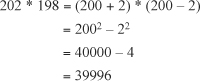
In addition to those that factor to exact squares, another kind of quadratic expression involves the difference of two squares. Consider the expression x2 – 25. This expression factors neatly as (x – 5)(x + 5). How it factors provides a reliable model for approaching all such factorizations. If you want to multiply two numbers that differ by a small amount, you can do it by squaring the average of the two numbers and subtracting the square of half the difference. Here is an example:
It’s possible to solve higher-degree polynomials, too, although it involves a little more work. Consider, for example, cubic functions. A cubic function (or equation) always has at least one root (a value x such that f(x) = 0). It can have up to three. The standard form of a cubic function is Ax3 + Bx2 + Cx + D = 0. The term D is referred to as the discriminant.
As with quadratic equations, you can find a solution to the cubic equation by finding a simpler equation. For starters, you find a quadratic equation that you can solve using the methods previously mentioned. For example, start by dividing the equation by A to obtain a simpler equation x3 + ax2 + bx + c = 0. Then make a substitution, replacing the variable x with a new variable t such that ![]() . This results in a new cubic equation with no quadratic term:
. This results in a new cubic equation with no quadratic term:
As before, the key to solving this cubic is the discriminant, D, where D = p3 + q2. Consider these notions:
If D > 0, then the equation has exactly one real root, the value r + s, where
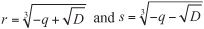 .
.If D = 0, then the equation has two roots,
 (a double root).
If D < 0, then you can find the three roots by using a trigonometric function. This is not covered until the next chapter, but for reference, the roots are given by

Having found values for t, you can then transform these into values for x by taking ![]() again.
again.
As you can see, this process is complicated. On the other hand, it is predictable enough to serve as the basis of an algorithm. From the algorithm, a reliable programming function can be generated. Here is one approach to such a function:
function solveCubic(a,b,c,d)
// d is the coefficient of the cubic term, the default being 1
if d is defined then divide a, b and c by d
set p to b/3 - a*a/9
set q to a*a*a/27—a*b/6 + c/2
set disc to p*p*p + q*q
if disc>=0 then
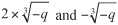
set r to cubeRoot(-q+sqrt(disc))
if disc=0 then set ret to [2*r, -r]
otherwise
set s to cubeRoot(-q-sqrt(disc))
set ret to [r+s]
end if
otherwise
set ang to acos(-q/sqrt(-p*p*p))
set r to 2*sqrt(-p)
set ret to an empty array
repeat for k=-1 to 1
set theta to (ang—2*pi*k)/3
append r*cos(theta) to ret
end repeat
end if
subtract a/3 from each element of ret
return ret
end function
There are two approaches generally used to solve equations. One is by substitution. The other is by elimination. Both approaches are usually interchangeable, but there are many instances in which you are likely to prefer one over the other.
If you have more than one unknown in an equation, it is not generally possible to determine them both. For example, if x + y = 5, then x could be 1 and y could be 4, or x could be 10 and y could be –5. An infinite number of other combinations are possible. However, if you have more information, such as another equation, it may be possible to find both unknowns. In general, if you have n unknowns, then you need n independent equations to find them. (An independent equation is one that cannot be deduced from the starting equation.) Fewer than n equations will not give you enough information, and more than n equations might give you too much information. If you have too little or too much information, you cannot solve the equations consistently.
A set of equations with the same unknowns is called a set of simultaneous equations. To explore this, first consider how you might solve a pair of simultaneous equations in two unknowns.
As a set of equations, suppose you start with the following:
x + 3y = 10
5x – 2y = –1
There are several ways to solve this set of equations. The first is by substitution. With substitution, you use one equation to find the value of one unknown as a function of the other. Then you substitute this value into the second. In this case, if you rearrange equation 1, you get x = 10 – 3y. If you then substitute this value into equation 2, you get

This process is called eliminating x. Generally, you use one equation in order to make a new equation for y that doesn’t involve x. Having found the value of y, you use the function for x: x = 10 – 3y = 10 – 9 = 1. If you substitute these values for x and y back into equation 2, you get 5x – 2y = 5 – 6 = –1.
The substitution method is most useful when dealing with non-linear equations. Such equations involve such terms as x2, y2 or xy. To explore substitution further, consider this set of equations:
3x + 2 xy = 7
2x + 5y – y2 = 8
Examining the first equation, you can see that you can factor the left-hand side to get x(3 + 2y) = 7, which means that ![]() You can now substitute this value into the second equation, which allows you to arrive at a cubic equation as follows:
You can now substitute this value into the second equation, which allows you to arrive at a cubic equation as follows:
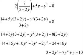
Given that you have reached a cubic equation, you have a clear path to a solution. In this case, the solution is made simpler because you can see it by inspection. If you substitute the value y = –1 into the expression on the right, you get the answer, 0. This means that the expression (y + 1) must be a factor. [This is an example of a general theorem, which says that if a is a root of a function f(x), then (x – 1) is a factor of the function. Recall that a root is expressed as f(a) = 0.]
To factor a polynomial expression when you know one of the factors is a simple task. You just take it one step at a time. Consider the equation arrived at so far, 2y3 – 7y2 + y + 10. If you know one of the factors, then you can express the problem as 2y3 – 7y2 + y + 10 = (y + 1)(...). You then proceed to find the expression inside the parentheses. Toward this goal, the first term in the parentheses must be 2y2, and the first term when expanded will be 2y3. This means that the factors can be expressed as (y + 1)(2y2 +...).
If you try expanding this tentative expression, you get 2y3 + 2y2 + ..., but the term in y2 should actually be –7y2. You need another term, –9y2, to make up the difference. This means that you now have the tentative factorization (y + 1)(2y2 –9y + ...). Again, if you expand this expression, you arrive at 2y3 – 7y2 + 9y + .... Now you need to match the coefficient of y, which should be 1. To get this, you must add another 10 y to the answer, which means your final factorization is (y + 1)(2y2 – 9y + 10). When you multiply out the terms in the parentheses, you get the answer.
Now you have a quadratic function, and you can factor it as before. To do this, you require two numbers whose product is 20 and whose sum is –9. These are –5 and –4. This gives you these factors: (y + 1)(y – 2)(2y – 5).
You are almost there! From the previous factorization of the cubic equation, you now know that there are three possible values for y: y = –1, y = 2, or y = 5/2. For each of these values, you can substitute back into equation 1, to get three possible pairs of values x and y: (7,–1), (1,2), or (⅞, 5/2). Substituting any of these pairs into equation 2, you arrive at the answer, 8.
If the process seems exhausting, one explanation is that the problem is more difficult than many others. Working with a difficult problem is worthwhile, however, because such a problem reveals how helpful the substitution method can be.
In addition to substitution, simultaneous equations can be solved using elimination. To see how this is so, consider a new pair of linear simultaneous equations in two variables:
3x + 2y = 2
2x + 5y = 16
While this system of equations could be solved using substitution, you can also add multiples of the equations together. Given that you know that a = b, and that c = d, you can add together linear sums of the equations and get a new equation, such as 2a + 3c = 2b + 3b. This process can be used to eliminate a particular variable.
Accordingly, if you multiply the first equation by 2, you get
6x + 4y = 4
and if you multiply the second one by 3, you get
6x + 15y = 48
If you then subtract the first of these new equations from the second, the result is an equation in y, which is

You can then substitute this value back into equation 1, getting

How do you determine the values used to multiply the two equations? It’s the same process involved in finding a common denominator. If you want to eliminate the variable x, your goal is to put the two equations over the common denominator of the coefficients of x. In this case, the common denominator of 3 and 2 is 6. As with fractions, you then multiply each equation by the common denominator divided by the coefficient of x in the equation.
To explore this further, here is another example:
Subtracting equation 3 from equation 4, you arrive at
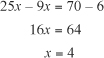
Substituting back in equation 1, you get

Check by substituting both values back into equation 2:
Elimination is used generally to solve any system of linear simultaneous equations. As a demonstration of how this is so, one approach is to develop an algorithm and write code to implement it.
Suppose you have n linear equations in n variables. You can write each equation as an n + 1 element array. For example, 2x + 3y = 3 becomes [2,3,3]. The complete system of equations is then an array of n such arrays, which can be represented as a function parameter simul. To solve the system of equations, the following function can then be developed:
function solveSimultaneous(simul)
   set redux to an empty array
   set n to the number of elements of simul
   repeat for i=n down to 1
      repeat for j=i down to 1
         if simul[j][i] is not 0 then
            set row=simul[j] and quit this loop
         end if
      end repeat
      if no row found then return "no unique solution"
      divide row by row[i]
      add row to redux
      delete row from simul
      repeat for j=i-1 down to 1
         if simul[j][i] is not 0 then
            subtract row*simul[j][i] from simul[j]
         end if
      end repeat
   end repeat
   set output to an array with n elements
   repeat for i =n down to 1
      set sum to 0
      repeat for j=i +1 to n
         add redux[i][j]*output[j] to sum
      end repeat
      set output[i] to redux[i][n+1]-sum
   end repeat
   return output
end
The solveSimultaneous() function uses an algorithm that has two parts. First, it goes through the equations one by one, at each step picking an equation with a target coefficient. Say that you are working in three variables, x, y, z, and the current variable is x. Such an equation might be 2x + 4y + z = 8. You divide this equation by the coefficient of x to give it a coefficient of ![]() . The resulting equation is added to a list of of reduced equations. (Such a list is called the redux.) Then you subtract multiples of the equation from all the remaining equations to eliminate the variable x from each.
. The resulting equation is added to a list of of reduced equations. (Such a list is called the redux.) Then you subtract multiples of the equation from all the remaining equations to eliminate the variable x from each.
Suppose one of the equations is 3x – z = 5. You subtract 3 times the equation from it in order to eliminate x, getting ![]() . While this specific step eliminates x from the equation, it has also brought y into it once again. This is not a problem. The goal is to eliminate x. At the end of the process, you have an equation in redux with a coefficient of 1 in x, and all the remaining equations in
. While this specific step eliminates x from the equation, it has also brought y into it once again. This is not a problem. The goal is to eliminate x. At the end of the process, you have an equation in redux with a coefficient of 1 in x, and all the remaining equations in simul have a zero coefficient in x.
If at any stage you can’t find an equation with a non-zero coefficient in the current variable, then you are stuck. The n equations are not independent. In this case, there are two possibilities: either there is no solution to the equations, or there are an infinite number of solutions.
When you repeat this process for y and z, you end up with a set of equations in redux with the following properties:
The ith equation has zero coefficients for the first (i – 1) variable.
The ith equation has a 1 coefficient for the ith variable.
The second stage of the process uses this information to solve the equations. The solution arises from working backward. Notice that the final equation is simple. Since it tells you the value of the last variable, which is something like z = 2, you can write this number into the output. Now you look at the second-to-last equation, which is something like y – 2z = 3. Since you know the value of z, you can substitute it into the equation and quickly find y. In this case, y is 7. You keep working backward through the equations, and at each stage you find the current unknown by substituting for all the later variables.
Simultaneous equations come up a lot in physics, particularly the collision detection calculations. While they might serve as the topic of a much more extended discussion, however, at this point it is important to move on to another central concern of algebra, one that involves visualizing the behavior of functions.
This section explores functions and how they can be used. One of the most prevalent uses of functions is to generate visualizations, and graphs are the primary form of visualization.
A graph is a way of representing data visually. The standard form of graph is the two-dimensional Cartesian graph, which displays all possible ordered pairs of two numbers in the form of points drawn on a flat sheet or Cartesian plane. To make a Cartesian plane, you need three things: an origin, which is a single point that you define as representing the point (0, 0), and two axes, (pronounced ax-ease, the plural of the word axis). An axis is a direction on the plane, and it is drawn as a line through the origin, with arrows to indicate the directions. The values plotted on the axes can be negative or positive. Those above or to the right of the origin are positive, and those to the left or below the origin are negative. The arrows indicate that the values in all directions continue to infinity. Figure 3.1 shows an empty Cartesian plane.

For the Cartesian plane to represent pairs of numbers, each axis must correspond to one number in the pair. While the horizontal axis represents the first number, the vertical axis represents the second. The two axes are usually labeled as x and y and drawn at right angles to one another. As illustrated by Figure 3.2, if you assign each axis a scale, then any pair of numbers (a, b) can be represented by measuring a distance a in the direction of the first axis, and a distance b in the direction of the second axis. This process is called plotting the point (a, b), and the values a and b are called coordinates. If the axes are x and y, then a is the x-coordinate, and b is the y-coordinate.
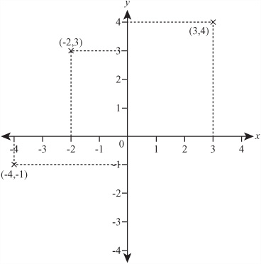
You can also follow the opposite process, reading the value of a point P on the plane. If you draw a line through P, perpendicular to the x-axis, it has to meet the y-axis at some point Q. As illustrated by Figure 3.3, if you measure the distance from Q to P in the scale of the x-axis, this will give you the x-coordinate of P, and if you measure the distance from the origin (often abbreviated as O) to Q in the scale of the y-axis, this will give you the y-coordinate. Note that the point P has been marked, and P is the point (2, 4).

Graphs are most useful for representing functions. If you have a function f(x), then you can represent it on a graph by taking every possible value of x, finding the value of f(x), and plotting the point (x, f(x)). Generally, you plot the variable along the horizontal axis and the output of the function on the vertical axis. A common expression of this is plotting f(x) against x. Alternatively, you can label the vertical axis with y and say that you are plotting the graph of y = f(x). If f(x) = 2x + 1, then you are plotting the graph of y = 2x + 1.
Note
In this chapter, functions in one variable are discussed. However, it is perfectly possible to make a graph of a function in more than one variable. Such graphs are difficult to create on a piece of paper. To draw a function in two variables, a three-dimensional graph (or surface) is required. Tools such as MATLAB make working with 3-dimensional graphs fairly easy. To draw a function with four or more variables, you need a graph with four or more dimensions. With these, also, mathematical software is extremely helpful.
It’s fairly straightforward to make the computer draw a graph. The precise details depend on the classes or functions that a given programming language offers. The drawGraph() function draws a graph on the basis of another function passed to it as a parameter along with a range of values for x. Representing the number of evenly spaced values of x to be plotted, the resolution parameter is used to determine how accurately the graph is drawn. It will also automatically scale the y-axis to fit the entire function into the graph. The dimensions of the graph are passed in as the last two parameters, and the graph is always drawn to include both axes.
Note
The graphics functions of most programming languages represent point (0,0) at the upper left of the screen and draw to the right and downward from it. This approach differs from how people are usually taught to draw graphs. In this drawGraph() function, these details are ignored; it simply plots a point or draws a line. To make it plot a line or figure relative to the origin of the axes, you must translate the value to the coordinate plane.
function drawGraph(functionToDraw, minX, maxX, resolution, width, height)
   // calculate values of the function
   set xValues to an empty array
   set yValues to an empty array
   set spacing to (maxX—minX) / (resolution - 1)
   // spacing is the distance between consecutive x values
   repeat for i = 0 to (resolution–1)
      set x to minX + i * spacing
      set y to calculateValue(functionToDraw(x))
      // how this is done depends on how you want to represent
      // the function. In the version on the CD-ROM, you can
      // pass either a string such as "x*x + 2*x + 3" or the
      // name of any function defined somewhere. The latter is
      // more flexible as it allows you to deal with special

      // cases such as "undefined" (see later in the function)
      append x to xValues
      append y to yValues
   end repeat

   // calculate the scale of the graph
   set leftX to min(minX, 0)
   set rightX to max(maxX, 0)
   // leftX and rightX are the x-values at each end of the
   // x-axis to be drawn
   set xScale to width / (rightX - leftX)
   set topY to max(largest(yValues), 0)
   set bottomY to min(smallest(yValues) , 0)
   // largest() and smallest() should return the largest and
   // smallest values in the array respectively
   set yScale to height / (topY—bottomY)

   // draw axes
   set x0 to xScale * (-leftX)
   set y0 to yScale * (-bottomY)
   // x0 and y0 are the positions within the graph of the axes
   draw a line from the point (x0, 0) to the point (x0, height)
   // this is the y-axis—you should also add arrows,
   // a scale and labels here
   draw a line from the point (0, y0) to the point (width, y0)
   // this is the x-axis

   // draw the function
   set currentPoint to 0
   repeat for i = 1 to the number of elements in xValues
      set x to xValues[i]
      set y to yValues[i]
      if y = "undefined" then
         set currentPoint to 0
      otherwise
         set thisPoint to ((x—leftX)* xScale, (y-ybottom) * yScale)
         if currentPoint = 0 then
            plot the point thisPoint
         otherwise
            draw a line from currentPoint to thisPoint

            end if
            set currentPoint to thisPoint
         end if
      end repeat
   end
Figure 3.4 provides samples of the output that drawGraph() function might generate. The version of the function used to generated Figure 3.4 provides labeling of the plots. You can access this function in the code for this chapter provided on the book’s companion website.

As rudimentary as the output of the drawGraph() function is, it is still valuable as a template or creating functions that generate graphs. The chief characteristics are as follows:
The horizontal line represents the equation y = 15. This equation is based on the constant function f(x) = 15, which returns 15 regardless of the value of x. You can also draw a vertical line with the equation x = c. As an example, the y-axis is drawn along the line x = 0.
The diagonal straight line represents the equation y = 2 x + 1, illustrating why a function with only a constant term and a term in x is called linear. All such functions appear as a straight line graph.
The curve, which looks like a big U-shape, is called a parabola. It represents the equation y = 4x2 – 16. All quadratic functions produce a similar shape. If the term in x2 is negative, the curve is inverted.
The two curves that hug the axes of the graph, sloping upward and to the right or downward and to the left and disappearing off to infinity near the axes, is the graph of
 . As x gets closer and closer to
  gets very large. In fact, it gets arbitrarily large, and the general expression for this is that it tends to infinity. Similarly, as x increases to infinity, y gets smaller and smaller, without ever quite reaching 0. When you see this behavior, you say that the lines x = 0 and y = 0 are asymptotes of the function.
While plots of graphs don’t tell you anything new about functions, they are of inestimable value in almost any mathematical, scientific, and technical context. Among other things, they allow certain important pieces of data to be seen quickly. Consider, for example, the questions of whether or where the line passes through the axes. Does it reach a maximum value or minimum value? Does it go off to infinity? Does it have asymptotes? As importantly, you can use this information to deduce other facts about the function. To explore such questions, consider what the graphs plotted in Figure 3.4 allow you to determine about the functions.
The horizontal line has two main features. First, it is horizontal, which means that it is a constant function, independent of x. Second, it crosses the x-axis at y = 3. These two facts tell you everything that can be said about the function. It is a constant function, and all such functions behave in a similar way.
The diagonal line can be described in various ways, but the two most important are the gradient and the intercept. The gradient of a straight line is defined the same way as the gradient of a hill. If you travel a certain horizontal distance, you also travel a certain distance upward. The ratio of these two values, vertical to horizontal, is the gradient. You can measure the gradient by taking any two points on the line and dividing the vertical distance between them by the horizontal distance. In this case, the line passes through the points (2, 5) and (–0.5, 0), which are separated by 5 units vertically and 2.5 units horizontally. If you divide 5 by 2.5, you get a gradient of 2.
The intercept is the point at which the line crosses the y-axis, which in this case is y = 1. Another thing to notice about these values is that when you look at the equation of the line, y = 2x + 1, you see that 2 is the gradient and 1 is the intercept. This is a general fact about straight-line graphs. The gradient is the coefficient of the x term, and the intercept is a constant value. The gradient is often represented by the parameter m and the intercept by c. Given this characterization, the family of linear equations is represented by the equation y = mx + c.
Parabolas offer more information than horizontal and diagonal lines. First, as mentioned previously, they can either curve downward, like a bowl, or upward, like a mountain. This gives you the sign of the term in x2. A bowl has a positive coefficient of x2, and a mountain has a negative coefficient.
Second, by observing the points at which the parabola intersects the x-axis, you can determine the roots of the function. [Recall that a root of a function f(x) is a value a such that f(a) is zero.] In this case, the curve crosses the x-axis at +2 and –2, showing that the roots of the function are +2 and –2. This means that (x + 2) and (x – 2) are the factors of the function. If the parabola only just touches the x-axis, then you have a function with just one root. This means that the function is a square quadratic. If it doesn’t cross the x-axis at all, then the function has no real roots and cannot be factored.
A third point is that, as with the straight line, you can determine the constant term of the function from the point at which it crosses the y-axis. A final point is that you can find the maximum or minimum value of the function from the curve, by locating the point at which the parabola turns back on itself and reading the y-value at that point.
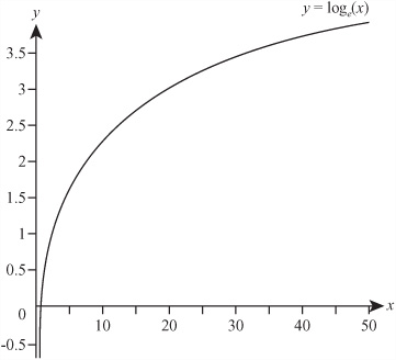
The function ![]() generates asymptotes. Such functions are harder to characterize or read information from than are the others, but you can read off the values of the asymptotes directly. Caution is necessary, however. Many functions that seem to have asymptotes are actually just changing very slowly. Consider, for example, the graph in Figure 3.5 of y = loge(x). The logarithm function does not have a maximum value, although from the graph it may seem that it does.
generates asymptotes. Such functions are harder to characterize or read information from than are the others, but you can read off the values of the asymptotes directly. Caution is necessary, however. Many functions that seem to have asymptotes are actually just changing very slowly. Consider, for example, the graph in Figure 3.5 of y = loge(x). The logarithm function does not have a maximum value, although from the graph it may seem that it does.
Although simple functions are the most common things to draw on a graph, not all curves can be described in terms of a standard function. The graphs you have seen so far have been of single-valued functions. It is not possible to draw a circle using this technique because a circle does not have a distinct value of y for each x-coordinate. In terms of functions, a circle is multivalued.
One way to avoid the problem created by multivalued functions is to use a parameterization. When you do this, instead of using a single function f(x) and plotting y = f(x), you use two functions x(t) and y(t) and plot the points (x(t), y(t)) for each value of t. The token t serves as a dummy variable here. However, because parametric functions are often used to represent motion and motion involves time, t frequently represents time.
To illustrate how parametric equations work, suppose that two functions are given by the formulas x = at2 and y = 2at. If you plot a graph of the points (x,y) given by allowing t to vary across the real numbers, you get the graph shown in Figure 3.6, which is a parabola lying on its side. In fact, it’s the parabola y2= 4ax, as you can find by substituting for t in the parametric formula.

This curve is one that you couldn’t draw using the drawGraph() function, because it’s multivalued in the y-coordinate. As you’ll see in later chapters, parametric formulas allow you to draw far more complex curves than simple functions, including the Bezier curves and splines seen in vector drawing and 3D modeling packages.
Write a function named substitute(functionString, x) that substitutes a value for x into a function given in standard notation.
The function should take two arguments, a string such as “5x^2 + 3(4-2x)” and a value such as 5, and should return the result of substituting the second argument for the variable x in the string. Use the ^ character as shown previously to represent powers, and the / and * characters to represent division and multiplication. Try to make the function as general as possible, particularly dealing with parentheses. Here are a few test functions you could try it out on: 5x + 3, 4 - 2(x-5), (x^3-4)/2, (x - 4)(2 - 3x), 2^(x - 4)/(x - 5)).
Write a function named simplify(functionString), which simplifies a given function as far as it can.
Simplification is a task requiring intelligence, and you won’t be able to make the function work as well as a human would, but you should be able to make some headway. Your program should be able to take a function, group like terms together, put fractions over a common denominator, and if you are very ambitious, factorize the result. You could work just with the variable x, or allow multiple variables.
In the course of this chapter, you have covered several years’ worth of basic algebra, which necessarily means you have missed out on many details and lots of practice. On the other hand, applying programming techniques to the concepts will have given you a good head start in understanding them.
The methods and concepts involved have been presented in an advanced fashion. The key focus of the discussion has been keeping the idea of the function at the forefront. As long as you understand what a function is, the rest of algebra falls neatly into place.
In the next chapter, you’ll slow down a little and begin looking at geometry, another topic directly relevant to programming.
The meanings of the terms variable, parameter, constant, and unknown and how they are related to and different from each other
The meaning of the word function, the idea of a function as a map between different sets, and the concepts of one-to-one, many-to-one, and multivalued functions
What an equation is and how to solve one for a particular unknown in simple cases, including quadratics, cubics, and simultaneous equations in two or more unknowns
How to simplify and factor functions, and use these skills to help with solving equations
How to draw a graph of a function, and how to use it to read off information about the function
How to draw a parametric curve