
This is the final chapter on 3-D graphics. It examines techniques for creating complex objects at the mesh level. So far, you’ve been looking at how to move objects from place to place without considering how they are made. You have assumed that the objects are either primitives, such as spheres or boxes, or pre-existing polygonal meshes. At this point, you will examine underlying surfaces and how they can be defined. You’re also going to explore surfaces, such as water and cloth, that can be animated in real time, and you’ll finish up with a brief look at creating animated characters.
The discussion includes attention to inverse kinematics, a technique for animation that has become popular due to its use in different animation tools. Since you will be examining the mathematics behind the technology, most of the topics in this chapter are advanced. It is important to remember this. While you will gain familiarity with mathematical and technical topics discussed, whole books have been written to treat the topics introduced. In this respect, it is hoped that this chapter will leave you with enough knowledge to be curious about further research.
A good beginning for a discussion of 3-D modeling is static modeling. Static modeling concerns how you can build a realistic-looking surface from simple parts.
Among other things, you can employ lathe technique to create a surface. The lathe technique involves creating a surface of rotation. To create a surface of rotation, you begin by defining a function f in one variable, usually one that does not have any roots in a particular interval. You then define your surface as the set of 3-D points whose distance from the x-axis at a particular value of x is f(x) over some range of x-values. As illustrated by Figure 21.1, given the use of a particular cubic function, the resulting surface is shaped like a vase. The plot of the path is made on either side of an axis, and by revolving the function plot around the axis, a 3-D shape is generated. This, then, is a surface of revolution.

A surprising number of useful shapes can be created as surfaces of revolution. You can generate anything with complete rotational symmetry along one axis. This implies anything can be modeled on a potter’s wheel. The big advantage of this approach is that many physical elements become reasonably easy to deal with. Among other things, the moment of inertia of a surface of revolution about its axis of symmetry is proportional to the integral of the function used for the revolution, ![]() .
.
Similarly, collision detection with a surface of revolution, while not simple, is somewhat simplified. You can consider the surface to be a succession of frusta of cones, and you’re interested only in collisions along the main surface, not with the top or bottom, which are the cause of most complications.
To create more complex surfaces, your best bet is to extend the concept of a spline into three dimensions, creating a spline surface. It will be necessary to review several topics before getting the whole story on how this is accomplished, for the spline surface of choice in 3-D is the B-spline, or NURBS (which stands for non-uniform rational B-spline), and this proves to be a fairly complex mathematical topic. However, with reference to topics previously discussed, one beginning is to consider how you might extend the concept of a Bezier or Catmull-Rom spline into 3-D.
The simplest application is to create a single curve in space, giving it some depth by defining a normal at each control point. As shown in Figure 21.2, the result is something like a 3-D track curving and twisting through space. Here, the main curve follows a standard Catmull-Rom spline, which makes each control point a 3-D vector. However, a second “virtual” Catmull-Rom spline in one dimension defines a curve of angles from the vertical. To accomplish this you associate an angle with each control point and then create a normal vector at each point that is both perpendicular to the curve and at the correct angle to the vertical. The result is a smooth track in 3-D.
Note
You’ll return to this example in Chapter 23, when you look at tiled 3-D splines.
The problem with the method depicted in Figure 21.2 is that it doesn’t enable you to create a complete surface. You end up with a surface that merely follows a specific line. However, you can overcome this limitation by creating a grid of curves instead. Toward this end, you define n × m control points and then use splines to interpolate a grid of n splines in one direction and m in the other. While it works fine for the purposes set, using this approach requires quite a lot of calculation, and the result offers no real integration of the two directions into one.
While the approaches discussed in the previous sections offer excellent beginning strategies for dealing with surfaces, in industrial contexts, surfaces are dealt with using different, more advanced approaches. The most common utility for drawing surfaces in 3-D packages is NURBS. Encompassing both Bezier and Catmull-Rom curves, B-splines are an extremely versatile form of spline. They can readily represent circles, ellipses, spheres, and tori, among other familiar shapes.
Note
A torus is a doughnut shape. The plural of torus is tori.
Unlike the splines you’ve looked at up to now, B-splines are not defined segment by segment as individual cubic curves. Instead, they are created by a single knot vector defined using a set of values {t0, t1, ..., tm} such that for each i < m, 0 ≤ ti ≤ ti+1 ≤ 1. This creates a set of points on the curve called knots, each of which is the result of setting the parameter t to one of the knot vector values.
Because different kinds of knot vectors create curves with particular kinds of behavior, the knot vector is the principal way to classify B-spline curves. When the knots are evenly spaced, the curve is called uniform. This is the source of the “non-uniform” (NU) in NURBS. However, in addition to knots, the physical shape of the curve is created by a number of control points, {P0, P1, ..., Pn}, where n ≤ m. You define the degree of your spline to be equal to k = m – n – 1.
One additional element is needed. This is a set of functions called the basis or blending functions. They are defined by a recursive process.
First, for p < j ≤ k, with ![]() defined as 0, you have the following equation:
defined as 0, you have the following equation:
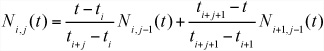
Then, for ti ≤ t ≤ ti+1 (and otherwise 0), you have
Ni,0(t) = 1
Note
Recall the definition basis from the world of vectors. As it happens, it’s possible to extend the concept of a vector space into more abstract realms, particularly that of functions. Just as with more conventional vectors, a basis in an abstract vector space is a set of elements such that any element of the space can be written uniquely as a linear sum of multiples of the basis elements. As a result, a basis for the space of polynomial functions might be the functions 1, x, x2, x3, and so on. This space has an infinite number of dimensions.
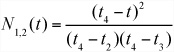
Since these functions are a little hard to visualize, it might help to introduce a simple example. Suppose that you have five knots at 0, 0.2, 0.5, 0.8, and 1 and a curve of degree 2 (so it has two control points) for which you want to find N1,2. By the recursive definition, you have
Applying the definition again, you get

Now you have reduced all the functions to j = 0, which means you can now apply the elementary definition, giving you several different behaviors enumerated in the following list:
If t < 0.2, then all of the functions evaluate to 0, and you have N1,2(t) = 0.
If 0.2 ≤ t < 0.5, then you have N1,0(t) = 1, so

If 0.5 ≤ t < 0.8, then you have N2,0(t) = 1, so

If 0.8 ≤ t < 1, then you have N3,0(t) = 1, so
Notice that if j = k, then the basis functions contain a reference to k + 1 of the function Ni,0. Notice also that the functions are entirely independent of the values of the control points. This is the reason that the knot vector has such a profound impact on the behavior of the curve. Further, although the definitions of the basis functions seem involved, computationally they are quite simple. The NURBSbasisFunction() function encapsulates the recursion involved in the computation in relatively few lines of code:
function NURBSbasisFunction( i, j, t, knotvector)
   if j=0 then // bottom out recursion
      if t<knotvector[i+1] then return 0
      if t>=knotvector[i+2] then return 0
      return 1
   end if
   // otherwise recurse
   if (knotvector[i+j+1]-knotvector[i+1])=0 then set a to 0
      otherwise set a to (t-knotvector[i+1]) /
                  (knotvector[i+j+1]-knotvector[i+1])
   if (knotvector[i+j+2]-knotvector[i+2])=0 then set b to 0
       otherwise set b to (knotvector[i+j+2]-t)/
                  (knotvector[i+j+2]-knotvector[i+2])
   return a*NURBSbasisFunction(i,j-1,t,knotvector)
            + b*NURBSbasisFunction(i+1,j-1,t,knotvector)
end function
Having defined the basis functions, you can at last arrive at the equation of the B-spline curve. It reads as follows:
While the function is easy to compute, notice that it is more abstract than the splines you’ve seen before. However, you still have a local behavior. Each curve segment is affected only by the nearby control points. In this case, each basis function, and thus each control point, contributes to exactly k + 1 of the curve segments.
A question remains, however. What about the rational B-spline (RBS) part of the NURBS acronym? Consider that if you use homogeneous coordinates to define your control points, you can think of the coordinates as a 3-D vector and a scalar wi, which is the weight of the control point. This can be done for all B-splines by setting wi to 1 for each control point. Allowing w to vary gives you a little more control. Curves in which w is always 1 are called non-rational. Curves in which w is allowed to vary are called rational. This leaves you with the general formula for a NURBS curve:

Note
NURBS is a singular noun, so you can speak of “a NURBS.” However, it is usually used as an adjective. You typically say, for example, “a NURBS surface” or “a NURBS curve.”
Rational B-splines provide one major advantage over NURBS. They are invariant under all transformations. If you transform space, objects on one side of the NURBS surface might not end up on the same side afterward. This is not so with a rational B-spline. With rational B-splines, they will always end up on the same side afterward. However, NURBS are invariant under affine transformations and all transforms.
One great advantage of the NURBS over other splines is the ease with which their transformational characteristics can be transferred to a surface instead of a line. This is communicated by adding a second sum:

Here, the control points are now arranged in a grid, with p in one direction and q in the other, and with two knot vectors of degree k and l, respectively. In Exercise 21.1, you are asked to translate this description into an explicit algorithm.
NURBS surfaces provide an excellent tool for creating generic solid objects, but in some circumstances effective alternatives are available. One alternative arrives when creating an infinite ground or a height map. A height map in 3-D is a function in two variables. For each value of x and z, it gives a single value y. Since you can use it to specify an entire ground surface with just a few bits of information, it is useful to have a simple method for creating such a function.
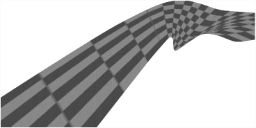
You’ve already seen one method for creating a height map. Presented in Chapter 15, that method used combinations of trigonometric functions. When several sine waves are combined, they produce a complex pattern. As shown in Figure 21.3, if you combine these in two directions, you end up with a random-seeming mountainous landscape.

A useful side-effect of combining trigonometric functions for generating a random landscape is that you can guarantee the maximum and minimum height of any mountain or valley. If you combine a number of waves, the maximum possible height for any mountain is just the sum of their amplitudes. Another advantage is that you don’t need to remember the height map for the whole landscape. The function is fixed in advance, so you can forget about distant areas and draw them at a later stage, without having to store them explicitly.
When you specify a surface algorithmically, you can describe a smooth, richly contoured surface without using an infinite number of points. In practice, however, your 3-D engine does not display a surface in such a graceful way. It must translate the surface into a set of polygons. But if you’ve stored your surface as a precise, infinitely smooth curve, this enables you to create a polygonal mesh at run time. This is a process called tessellation.
To tessellate a surface, you begin by calculating the coordinates of a number of points on the mesh. Usually, the points are uniformly spaced out along the s and t values for a NURBS surface. Either that, or they are spaced out along the x and z values for a ground surface, such as the trigonometric surface described previously. These values are then converted to a mesh by joining them into triangles. Depending on the 3-D API you are using, you can either send them as individual triangles or as a set of vertices and a set of values defining which vertices are to be connected with triangles. For example, DirectX allows you to define triangles as lists of three points, or as a “strip” of triangles, each of which extends the strip by one point, or as a “fan” of triangles emanating from a single point.
Given that you’re going to convert your surfaces to a mesh anyway, why not just store them as a mesh and be done with it? There are three principal reasons. The most obvious advantage is storage. Just as with the distinction between vector graphics and bitmaps, converting to a mesh generally requires less memory. In this case, you store a shape as a description rather than a predefined set of points. This is especially important when the shape is simple. If the shape is simple, then using NURBS is overkill, and you might be better off using an even simpler description. Consider, for example, an operation that can be described as “this is a sphere of radius 2.” On the other hand, if the shape is complex, like a character, or if it is naturally composed of polygons, like a jewel, then a polygon-by-polygon description might be more appropriate. In the middle ground, while a NURBS or similar system is likely to save on memory, it does increase the load time, for the engine must build the model using the formula.
Another advantage is scaling. Scaling allows you to choose how detailed your mesh will be. The detail of a mesh is usually known by its level of detail (LOD), and the level of detail refers to the number of polygons used in the construction of the mesh. If your end user has a fast machine, you can create a highly detailed mesh. On the other hand, if your end user has a slower machine, you can create a less detailed mesh. Either way, the polygons are still calculated by means of the same underlying curves, and this means that they will always be good approximations to the true surface. You can even choose to vary the LOD of the mesh according to how far away it is from the camera, as is done with a mip-map. In fact, LOD is used to describe different levels of mip-maps.
Many 3-D engines can calculate LOD meshes automatically, and may even perform the switch between them according to distance. You can sometimes tell in a game the moment at which a model in the distance changes its mesh to the simpler form.
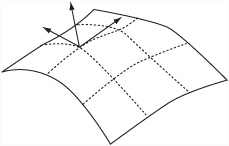
Scaling offers still another advantage. This advantage arises because scaling allows you to calculate the normal at a particular point on a surface generated algorithmically. You do this by using partial derivatives. (Partial derivatives were discussed in Chapter 6.) Use of this approach gives you two vectors tangential to the surface. As illustrated by Figure 21.4, you accomplish this by taking the cross product of these vectors. This gives you the normal.
In the case of a NURBS surface, the partial derivative of the basis functions in each direction can be described by a single polynomial of degree k – 1 (or l – 1). This gives you the constant for each knot span. You then can combine these partial derivatives into a partial derivative for the whole surface function. The outcome is that for each vertex of your mesh, in addition to calculating its position, you can calculate its normal. Similarly, you can calculate the normal for your trigonometric surface.
As with Bezier curves, mild advantages also accrue for these surfaces in collision detection, but the complications are large enough that using polygon-by-polygon collision detection is preferable.
Given that it’s reasonably simple to create it in real time, why not go the whole way and generate a complex surface from moment to moment, making a surface that can change over time? Several topics must be considered before an answer to this question can be given. These topics are the subject of the sections that follow.
Although it is fair enough to conclude that erotic appeal is the sole reason that over time characters in some games have been clothed in figure-hugging bodysuits, other reasons also apply. If the garments the characters wear hang loosely, the movement of the fabric must be calculated, and such calculations are computationally intensive. As a result, during much of the history of games, an incentive has existed to use loose clothing sparingly. However, as computers have increased in speed, loose clothing has posed less of a problem, and it has become feasible to introduce a variety of loose clothing made of flowing cloth, even in real time.
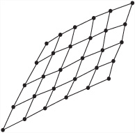
Cloth, hair, and skin pose challenges to developers that are continuously the occasion for new innovations. However, on a rudimentary level, a basic trick is used in their construction. As discussed in Chapter 16, this trick involves creating a system of coupled oscillators. As illustrated by Figure 21.5, a piece of cloth is essentially a grid of particles mutually connected by springs. You’ve already seen how to calculate the motion of a particle attached to a system of springs. Most physics APIs allow you to create virtual springs. However, you still need to consider how best to set up such a system.

To set a system of springs, one key consideration is that real-life cloth is usually woven from a set of interlocking fibers. Interlocking makes it so that the fibers behave differently when stretched in different directions. When a force is applied along the direction of the fibers along either the warp or the weft, the cloth scarcely stretches at all. When a force is applied to stretch the fibers along the bias or cross, directions that are diagonal to the fibers, the cloth stretches easily. The behavior of the cloth ends up being analogous to a garden trellis, as shown in Figure 21.6.
Cloth as modeled for animation can be pictured as a set of inextensible springs arranged in a lattice. Such springs are actually harder to simulate than ordinary springs. An inextensible spring is essentially the same as an extensive spring with an infinite coefficient of elasticity. On the computer, setting up such a spring, especially in a coupled lattice, leads almost instantly to major feedback problems. The feedback problem occurs because, as small errors accumulate, the whole simulation spirals out of control. Adding damping doesn’t help. In fact, damping tends to make the situation worse.
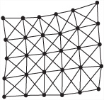
To overcome this problem, you must picture the cloth simulation as more like rubber. Rubber stretches equally in all directions. Using this analogy, as shown in Figure 21.7, you use springs to construct a lattice, as discussed previously, but this time you allow the springs a fairly high coefficient of elasticity. You also add cross-braces. The whole simulation is set up so that the natural length of the springs is the same as their length when the whole thing is flat.
To make the simulation more like skin rather than cloth, you can add an additional set of springs attaching each vertex to the underlying surface. These zero-length springs are sometimes called dashpots. In situations in which a surface is not the best medium, you join the springs in a chain. This approach is commonly used to simulate hair or a piece of rope.
Using the rubber surface method, you can create realistic cloth that hangs, flaps, and even drapes. For draping, you must include collision detection with the particles at the vertices. The only complication is user interaction. Because the mouse has no physical constraints in the simulated world, a user can easily create situations that are physically impossible. An example might be dragging a particle on a spring a long way past its elastic limit. Such problems can be solved fairly readily, however. In a situation in which the user can drag parts of the surface around, instead of having the user directly drag a particle, you can make is so that a force no greater than some set maximum on the particle is applied in a direction determined by the cursor. This will limit the amount by which the surface can move away from equilibrium.
In computer graphics, no great divide separates water and cloth. One approach you can use to create a realistic water surface involves a series of coupled oscillators. With the use of coupled oscillations, however, the forces underlying the coupling of the oscillations of nearby points on the surface of the water are quite complicated. They involve a combination of gravitation, pressure, and surface tension.
An alternative method, involves directly modeling the waves on the surface. As with the trigonometric surfaces you looked at before, a wavy surface can be defined by a series of wave functions that can be calculated independently. The height of the surface at a particular point is just the sum of all the waves at that point.
Using wave functions or oscillations, the accuracy you achieve in your modeling depends on the approach you use. With the simplest approach, you set up each vertex of the surface as an independent oscillator under simple harmonic motion (SHM). With this model, the various vertices should all move with the same frequency, but they can vary in amplitude and phase. The variation might be specified by a function or a texture map of some kind. This is a common form of simulating moving wave surfaces in games. While this system is simple to use and reasonably fast to calculate, one disadvantage is that it lacks flexibility, particularly in relation to user interactions. It isn’t affected by anything else that happens in the simulation.
If your goal is to make startlingly realistic waves, you can model them directly. The advantage of direct modeling is that the waves can then have different frequencies and can change over time. For example, simulating different weather conditions, you can make waves increase in strength over time. Waves on the surface can be of two kinds, simple parallel wavefronts moving in a straight line or circular wavefronts emanating from a point source, as happens when a pebble strikes the surface of a pond. Surface waves of either type allow you to create waves that respond to player actions.
All the methods mentioned so far create fake waves. They are fake because, among other things, they do not have crests or breakers. Crests and breakers occur when a wave moves from deep water to shallow water. When this happens, because it can’t drop to its lowest negative amplitude, the wave can no longer move symmetrically, so its energy is transferred to the top of the wave. With its energy transferred to the top, the wave moves forward instead of just up and down. To model such actions involves performing many calculations, and game developers often conclude that the processing power is not available in a realtime game to support such calculations. In the area of fluid dynamics, however, such calculations are essential. Likewise, such calculations are common in the film industry, where rendering is not accomplished on a real-time basis.
The final topic of this chapter concerns using bones to create animated characters. While modeling bone tools remove the need for animators to be involved in the details of bone creation, it remains important to delve into fundamentals if mathematical and programming operations are to be understood. This section explores the essential elements only.
The bone system has been around for a long while as a method for animating characters. It is all but universal. Using the bone system, a character is defined by a series of lines representing bones. As illustrated by Figure 21.8, these lines are arranged in a parent-child relationship. To create a model, the bones are fleshed out, and the model that results can be changed over time. Change involves rotating the bones. Each bone is rotated relative to its parent.
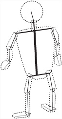
Since its surface must be modeled so that the skin doesn’t distort at the joints when a bone is flexed particularly far, the details of how a model using bones is created are quite subtle. Modeling software can do this kind of thing automatically. In the current context, however, it’s necessary only to think specifically about how bones work.
To start with, you create animation in a few basic ways. In one way, you use a pre-set series of motions, such as “run,” “jump,” “fall over,” and so on. These are often recorded by means of a motion capture system and a live model. In another way, you directly animate each bone in real time. With the pre-set approach, the work is much easier and tends to be the most commonly used. With the direct animation approach, the work is more involved and is often used for ragdoll animations. With ragdoll animations, the body of the character moves as a set of connected rods under gravity, without any muscle actions.
Because the joints of a model are constrained in various ways, creating a realistic ragdoll figure is difficult. For example, the human body includes ball-and-socket joints, such as the shoulder. These joints can swivel freely in two dimensions, with limited motion in the third. Other joints, like the knee, involve simple hinges that can rotate only in one dimension. The twisting motion of the forearm is achieved by using two separate bones rather than by motion in the elbow joint. Such constraints can be programmed using standard modeling packages, but to make them work in real time requires significant computational effort.
Making a ragdoll character move is essentially an exercise in kinematics. Kinematics is an area of physics that deals with the motions of systems without consideration of the physical laws accounting for the motions. With respect to character animation, kinematics deals with how the bones of a model are connected and move in relation to each other. To program kinematic actions, fairly extensive work is involved. The work combines rigid-body motion and 3-D collisions. The mathematical problems are usually solved numerically. With each time-frame, you can calculate the momentum and energy values and move the bones accordingly.
As an example of how kinematics works, consider a simple situation, illustrated by Figure 21.9, which provides a 2-D diagram. The system consists of two bones connected by a single pin. For each of the two bones, you know the current linear and angular velocity ui, ωi and the mass and moment of inertia mi, Ii. With 3-D animations, you would also need to know the moment of inertia about all three principal axes. For each bone, you assume that the pin is currently at a vector Xi from the center of the limb. All the motion occurs in two dimensions, but without any collisions, the limbs pass over or under one another.

It’s convenient to think in terms of the values ri = | xi | and ![]() . The values establish, respectively, the distance of the pin from the center and the clockwise vector tangential to the center, through the pin. The pinning of the various limbs implies at all times that the local velocity of these points of contact must be equal. You can calculate the local velocity of a particular point as a function of the motion of the limb:
. The values establish, respectively, the distance of the pin from the center and the clockwise vector tangential to the center, through the pin. The pinning of the various limbs implies at all times that the local velocity of these points of contact must be equal. You can calculate the local velocity of a particular point as a function of the motion of the limb:
At any time, this value must be equal for all pairs of bones at a particular pin. As presented in the following list, this reasoning gives you a set of equations for the new linear and angular velocities vi, φi:
From conservation of energy, you get

From conservation of linear and angular momentum (as long as there are no external collisions), you have two equations:

and

From the pinning, you get

Between them, these equations give four unknowns, two of which are vectors. Although it is not easy, the four unknowns can be solved. One reason for the difficulty is that neat division does not exist for radial and tangential parts.
One disadvantage to this formulation is that there is a tendency for numerical errors to creep in, making the various bones drift apart. An alternative formulation takes advantage of the parent-child relationship of the bones. This formulation considers one bone to be the root, with the other bone(s) slaved to it. All you need to know is the angular velocity of each bone about the pivot point with its parent. While this is a simpler and appropriate formulation, it is slightly harder to set up. It will not be further explored in this context.
A far more difficult task is the one that our brains accomplish every second of the day. This task involves controlling each bone of your body as you engage in one or another activity. What applies to your actions applies to that of a model as it is animated. The task of controlling the bones immediately leads to a major problem called inverse kinematics (IK). A question that someone working with inverse kinematics might ask is, “Which bones should I move to pick up a cup?”
Such questions are common and practical in the field of robotics, and what applies to robotics applies to animation. A wide variety of approaches have been made to solving such problems. As you will discover in Chapter 26, much interesting work has been done in this respect in the field of artificial intelligence (AI), especially as related to genetic algorithms. In this section, it is worthwhile to examine a few preliminary examples relating to inverse kinematics.
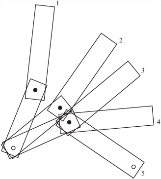
As a first example, consider the simplified bone illustrated in Figure 21.10. This model is similar to the one shown in Figure 21.9. It features a pair of jointed bones. The first bone, on the left, is fixed in place at its left end. The other end of the first bone can move freely. The second bone, which can move freely at both ends, is joined to the free end of the first bone. Suppose you want to reach the point P, touching it with the end point of the second bone.
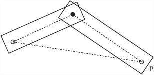
In Figure 21.10, finding the correct final configuration to meet P is reasonably easy. It involves application of the cosine rule. You can apply the cosine rule because you know the lengths of all three sides of the triangle formed by the joint and the end points. Even with this simple scheme, however, a few complications arise. In addition to finding the end point, you must work out the best route to reach it. Ideally, you want to minimize the amount of movement required to get from the initial configuration to the end configuration. As an example of how motion can be wasted, consider the positions illustrated by Figure 21.11.
One way to eliminate wasted motion is to create the complete motion path. To create a motion path, you attempt to move smoothly so that the free end of the second bone follows a simple line from its starting point to P, as shown in Figure 21.12. The advantage to this approach is that each movement is small and gets you progressively nearer to the goal. If the end-point is reachable, then this approach will always give a possible solution in the two-bone problem. However, it might not be physically possible if you are dealing with real characters with limited movement in the joints.

In case this seems to be overstressing the difficulty of working with inverse kinematics, remember that when there are more than two bones involved, typically there are an infinite number of possible configurations that solve the IK problem. Choosing the appropriate path for the bones is non-trivial. The best solution tends to result from an iterative approach to the solution, where the bones try to orient themselves toward the target a small amount at a time. One simple application of this method involves rotating each bone a little more toward the target at each time-step in proportion to how far away from the target it is currently. Exercise 21.2 poses this problem.
The same approach also works well in three dimensions, although it’s harder to make it work realistically because there are more degrees of freedom. It’s less successful when dealing with a system of bones that is not just a simple chain or when you need to worry about collision avoidance.
Create a program that will draw a 2-D NURBS. Your program should allow you to experiment with moving the control points around, changing the knot vector, and so on. If you’re feeling brave, try using a 3-D NURBS surface.
Create an iterative function IKapproach(chain, target) that adjusts a simple IK chain to hit a specified target. Your function should take a chain of bones specified in whatever way you prefer in a particular configuration and move it toward a particular target by some small amount. When applied successively, it should adjust the chain to hit the target.
To conclude the part of this book that discusses 3-D techniques, this chapter has led you through a brief discussion of methods dealing with surfaces. You have seen how you can use mathematical techniques to define a complex surface using various methods, especially B-splines, and how to make a surface with an adjustable level of detail. You’ve also looked at animated surfaces and bone systems. With the next chapter, you leave the subject of 3-D to spend the rest of the book looking at some algorithmic techniques, especially in the context of games.
How to define an object in 3-D in terms of a surface of revolution, NURBS, or trigonometric functions
How to use these mathematical descriptions to draw the object at different levels of detail
How to animate a surface to simulate water or cloth
How to create a bone system and use it to make a ragdoll simulation
Kinematics and how to solve simple inverse kinematic problems in two dimensions