Geometry is the study of shapes and space, and particularly of symmetry. In this chapter, you’ll look mostly at the practical side of the subject, however, beginning with the measurement of angles and triangles. This area of mathematics is trigonometry. When programming anything involving movement, such as games, you constantly use trigonometry. In fact, it is so important that you must have a thorough understanding of how it works.
An angle is a way to measuring a direction. If two people set off from the same point, after they have both traveled 10 meters, they can be anything from zero meters apart (if they set off in the same direction) to 20 meters apart (if they set off in opposite directions). An angle is a measurement of how different the two directions are.
The most common way to measure an angle is to consider the two possible directions as radii of a circle. You can then consider the angle between any two radii as a fraction of the circle. For example, in Figure 4.1, the clockwise angle between the lines A and B is a quarter of the circle, and the clockwise angle between the lines B and C is a third of the circle.

Note
A radius of a circle is a line from its center to its perimeter. Another term for perimeter is circumference. Radii is the plural of radius. If a straight line is drawn between two points on the circumference and passes through the center of the circle, it is called a diameter of the circle.
Since you can measure the angle in either direction, the phrase “the angle between two lines” is potentially ambiguous. In Figure 4.1, the counterclockwise angle between A and B is three quarters of the circle. Generally, when you talk of the angle between two lines, you mean the smallest angle. This will be the approach used in this chapter unless otherwise indicated. However, in later chapters, you’ll be more interested in measuring the angle in a particular direction.
Angles can be measured in different units, the most common of which is the degree. When measuring in degrees, you divide a full circle into 360 equal parts. Each part is a single degree, written as 1°. There is nothing special about 360, except that, as noted in Chapter 1, it has a large number of divisors, meaning that many common fractions of a circle have an integer number of degrees. Consider, for example, that a quarter turn is 90° (called a right angle), a half turn is 180° (a straight line), one third is 120°, a sixth is 60°, a fifth is 72°, and so on. Figure 4.2 illustrates some of these angles.

Figure 4.2. Some common angles measured in degrees. Measured angles are denoted by a small arc between the lines, and right angles are denoted by squares.
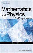
Of the angles shown in Figure 4.2, the most important is the right angle. A square has four equal sides, and the angle between each pair of adjacent sides is a right angle. If you draw the diagonals of the square, they also meet at right angles. When two straight lines meet at right angles, they are called perpendicular. Four right angles divide the circle into four equal quadrants. As illustrated by Figure 4.3, if a circle is drawn on a graph, the quadrants can be seen to be complimentary. For every point (x, y) inside the circle, there are corresponding points (x, –y), (–x, y) and (–x, –y). These are also inside the circle, each in a different quadrant—except when x or y is zero.
Certain terms facilitate discussion of the relative magnitudes of angles. An angle smaller than a right angle is called acute. An angle larger than a right angle (but smaller than two right angles) is called obtuse. An angle greater than half a circle is called a reflex angle.
If you draw a square around a circle and pick a point at random within it, what is the likelihood that this point lies inside the circle? This question is one way of explaining the concept of the area of a shape. Imagine that you have two squares, one that has sides twice as long as the sides of the other. You place the two squares side by side on a table. You then repeatedly make evenly spaced dots on the table with a pen. How many dots are within the respective squares? The answer is that four times as many dots are in the large square as in the smaller. The reason is that you can fit four of the small squares in the larger one, for four times as many dots appear in the larger square than in the smaller one. The notion of a unit squared extends this relationship. If a square has sides x units long, then the area of the square is x2 square units or units2 (hence the term squared). When x = 1, the shape is called a unit square.
You can easily calculate the area of a rectangle. Like a square, a rectangle is a shape that has four sides, and each pair of adjacent sides lies at right angles to each other. Unlike the four sides of a square, the four sides of a rectangle do not need to be equal. Only the sides that are opposite each other need to be equal. The implication is that a square is a special kind of rectangle. The area of a rectangle is the product of its length and width. The area of the rectangle in Figure 4.4 is 12 square units. In other words, 12 unit squares fit inside it.

You’ll return to areas when you look at triangles, but for now consider again the question that began this section. This question can be rephrased as, “What is the area of a circle?” To answer this question, it is necessary to first say specifically what is meant by a circle. A circle is the shape drawn when you hold the end of a piece of string at a fixed point, attach a pen to the other end, and draw a curve with the string held taut. The length of the string is the radius of the circle.
Note
The term radius refers both to a length and to a line. The radius of a circle is a line drawn from the center of a circle to its circumference, as mentioned earlier, but it is also the length of the line. Uses of radius are similar to those of side. For example, you might use the phrase “the side of a square” to mean “the length of each side of the square.” Likewise, you might use “the sides of a rectangle” to mean “the lengths of the two pairs of opposite sides of the rectangle.” Radius here means “the length of any radius.” Similarly, diameter can mean “the length of any diameter.”
Once you know the radius of a circle, you know almost everything there is to know about it, although you might also need to know the position of the center point. The area of a circle is always in a particular proportion to the square of its radius. If a circle has radius r, then it has an area of 3.1415927... × r2. The precise value of this constant 3.1415927... is given by the symbol π, which is the Greek equivalent of the letter “p,” spelled in English “pi” and pronounced “pie.” In many computer languages, this value can be accessed as a math property and is usually available either as a predefined constant PI or (less often) as function named pi().
π is probably the most ubiquitous irrational number in mathematics, cropping up in all kinds of unexpected places—even more than e, which runs a close second. Mathematicians have proved any number of surprising facts about this number over the centuries, with probably the most elegant provided by the mathematician Leibniz:
Involving a series similar to Leibniz’s, one of the earliest uses of computers on a vast scale was in calculating the digits of π to an enormous precision. Many terms of a series are required to get anywhere near to a precise value. Today the digits of π are known to over a trillion decimal places. This is testimony both to the importance of the number and to the obsessive nature of computer programmers.
If you know the formula for the area of the circle, you can answer the question concerning how to define a circle. A square drawn around a circle has a side equal to the diameter of the circle. If the circle has a radius of 1 unit, then the square has a side of 2 units and so an area of 4 units2. By the formula for the area of a circle, the circle has an area of π units2). So the circle has π/4 times the area of the square, which is a value of approximately 0.7854.
π also turns up in another important element of the circle, the length of its circumference. The circumference is equal to π times the length of the diameter, or π times twice the length of the radius.
As was emphasized previously, there is no particular reason for choosing the degree as a unit of angles. It is simply a unit that is convenient for some calculations. Although it may not seem very natural at first, another common unit of measurement is the radian. Instead of dividing a circle into 360 equal degrees, you divide it into 2π radians—which is to say, “six and a bit” of them. The idea of dividing the circle into non-integer units is what seems strange at first, but there is nothing wrong with it. After a while, it seems no odder than accepting the idea that there is not an exact number of centimeters in an inch.
It is often necessary to convert between degrees and radians. One radian is ![]() of a circle, so it is
of a circle, so it is ![]() degrees. Similarly, one degree is
degrees. Similarly, one degree is ![]() of a circle, so it is
of a circle, so it is ![]() radians. Thus an angle of 12° is equal to
radians. Thus an angle of 12° is equal to ![]() radians. An angle of
radians. An angle of ![]() radians is equal to 90°. If you must often convert between the values, it is generally simplest to store the conversion factor as a constant from the beginning.
radians is equal to 90°. If you must often convert between the values, it is generally simplest to store the conversion factor as a constant from the beginning.
There is a third unit of angles, which is called the gradian, but this is not something you are likely to encounter or need, although you can still find it on calculators. It is based on a division of the circle into 400 parts.
As was mentioned previously, trigonometry is the area of mathematics that studies triangles. At the same time, the triangle is also studied extensively as a subject of geometry. A triangle is a figure made up of three points not lying on a straight line that are joined by three straight-line segments. When points are positioned in this manner, they are known as non-collinear. Each point of the triangle is referred to as a vertex, and together they are the vertices of the triangle. When you apply algebra to trigonometry and geometry, the result is analytical geometry—a field of mathematics pioneered by Rene Descartes.
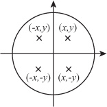
Triangles can be classified into four main types according to the three angles inside them. As illustrated in Figure 4.5, you normally identify the features of a triangle by using capital letters for vertices, lower-case letters for side lengths, and angles labeled either by Greek letters as in the figure or with an angle designation (such as ![]() ), listing three points that define the angle. Likewise, each side is labeled to correspond to the opposing vertex. You may also see the angles denoted simply by the letter of the vertex: angles A, B, or C. Small arcs are used to emphasize angles of the lines joined at the vertices.
), listing three points that define the angle. Likewise, each side is labeled to correspond to the opposing vertex. You may also see the angles denoted simply by the letter of the vertex: angles A, B, or C. Small arcs are used to emphasize angles of the lines joined at the vertices.
Note
If you are unfamiliar with the Greek alphabet, see Appendix C. For a quick review, however, note that α is alpha, β is beta, γ is gamma, δ is delta, e is epsilon, and θ is theta. You have already seen π (pi).
The angles of a triangle always add up to 180°. One demonstration of this is that if you draw the same triangle three times, as shown in Figure 4.6, you can see that the angles α, β, and γ lie on a straight line, which means that the sum of these angles must be half a circle, or 180°. That this is true for any triangle was demonstrated by Euclid (324 – 264 B.C.E.), the most famous of geometers, but has been known since the earliest days of geometry.

While a general set of propositions apply to all triangles, regardless of their shape, the shapes of triangles are classified according to the magnitudes of their angles. Generally, there are three classifications of triangles, as illustrated by Figure 4.7. The following list summarizes the three classifications.
Equilateral. The simplest triangle is the equilateral triangle, which has three equal sides and three equal angles. Given that angles of a triangle always equal 180°, each angle is equal to 60°.
Isosceles. An isosceles triangle has two equal sides. If sides a and b are equal, then angles α and β are also equal.
Scalene. A scalene triangle is any other triangle. Such triangles have no equal sides and no equal angles.

In addition to the three primary classifications of triangles, geometers refer to triangles as acute and obtuse. An obtuse triangle has one angle greater than 90°. An acute triangle has no angles greater than 90°. In this sense, then, equilateral and isosceles triangles are acute, and a scalene triangle is a candidate for being obtuse.
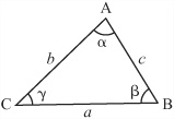
One particularly important kind of triangle the right-angled triangle. It is often referred to as a right triangle. As its names imply, it is a triangle that has a right angle within it. A right angle is an angle of 90°. There are special names for the sides of a right triangle. Two of the sides are called legs, and one is called the hypotenuse. As illustrated in Figure 4.8, two of the legs (a and b) are joined by a right angle (which is indicated by a small square or rectangle). The ends of the two legs are joined by the hypotenuse. Given that the right angle equals 90° and that the sum of the three angles must be 180°, the two smaller angles must necessarily sum to 90°.
The Greek mathematician and philosopher Pythagoras (569 – 494 B.C.E.) is famous for having developed a theorem that relates the sides of the right triangle. This is usually referred to as the Pythagorean Theorem. It was left for Rene Descartes (1596 – 1650) and other mathematicians to extend and apply the Pythagorean Theorem to the coordinate system and algebra.
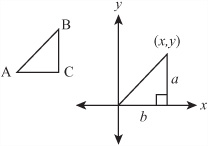
How the Pythagorean Theorem works begins with right-angled triangles. There are several reasons why such triangles are important. The first is that they are easy to recognize and crop up in many natural circumstances. For example, when working on a graph, it is often useful to draw the lines joining points and create a right-angled triangle with sides parallel to the x- and y-axes, as is shown in Figure 4.9. As was discussed in a previous chapter, the gradient, or slope, of a line is given by the ratio of the one side of the triangle (a) to another (b) or, on the x- and y-axes, the ratio of y to x (the run to the rise).
Triangle: Gradient (or slope) = a/b
Coordinate System: Gradient (or slope) = y/x
A second reason for the importance of right-angled triangles is that they have a number of useful properties. These will be dealt with in subsequent sections. A third reason, as Figure 4.10 illustrates, is that any triangle can be easily split into two right-angled triangles by dropping a perpendicular from one vertex to the opposing side.

Figure 4.10. A triangle split into two right-angled triangles by dropping a perpendicular from vertex A.
As mentioned already, right-angled triangles were studied extensively by Pythagoras. The Pythagorean Theorem states that for a right-angled triangle ABC with the right-angle at vertex C, a2 + b2 = c2. There are many ways to prove this theorem. One approach is shown in Figure 4.11.

In Figure 4.11, in the diagram on the left, you find a square with side a + b. Around the outside are arranged four equal right-angled triangles with legs a and b. The hypotenuses of the triangles, with length c, form a smaller square inside the larger, whose area is c2.
In the diagram on the right, you have an identical square, again with side a + b. This time, the four right-angled triangles have been rearranged to fit inside the square as two rectangles meeting at a corner. Each rectangle has sides a and b. The remainder of the square is subdivided into two smaller squares, one of which has side a, the other side b.
The total area of these two squares is a2 + b2. However, since these the two large squares and the eight right-angled triangles within them are all the same, the area of the two small squares in the diagram on the right must be equal to the area of the square in the diagram on the left. Given this observation, you can conclude, that a2 + b2 = c2.
There are an infinite number of right-angled triangles whose sides are of integer lengths. The smallest is the triangle with legs 3 and 4, which has hypotenuse 5. There are a number of ways of generating such triangles, and the sets of three numbers making the sides are called Pythagorean triples. There are no sets of integers for which the same is true in any higher power. In other words, there are no sets of positive integers a, b, c, n, with n>2, such that an + bn = cn. This fact is called Fermat’s Last Theorem and was a famous unsolved problem until very recently.
Using the Pythagorean Theorem, if you are given the lengths of the two sides of a right triangle, you can quickly determine the length of the third side. For example, if you know that the hypotenuse of a triangle is 13 cm, and one side is 5 cm, then by Pythagoras, the third side’s length must be equal to ![]() .
.
As illustrated by Figure 4.12, a right-angled isosceles triangle with sides that are half a square (usually referred to as unit length) has a hypotenuse ![]() units long. Similarly, if you take an equilateral triangle with sides of length 2 and cut it in half, the length of the perpendicular is
units long. Similarly, if you take an equilateral triangle with sides of length 2 and cut it in half, the length of the perpendicular is ![]() units. When this is done, notice that the isosceles triangle has interior angles of 45°, and the triangle with a perpendicular of
units. When this is done, notice that the isosceles triangle has interior angles of 45°, and the triangle with a perpendicular of ![]() units has angles of 60° and 30°.
units has angles of 60° and 30°.

Refer back to Figure 4.9 and note that the gradient (or slope) of a line can be can be represented by drawing a right-angled triangle on a graph. For any right-angled triangle with leg a parallel to the y-axis and leg b parallel to the x-axis, the gradient of the hypotenuse is equal to ![]() . It is useful to be able to relate this value to the size of the angles at A and B, and you do this by using the
. It is useful to be able to relate this value to the size of the angles at A and B, and you do this by using the tan() function. If the angle at A is x, then tan(x) gives the gradient of the line AB. Two other functions, sin(x) and cos(x) are equal to the ratios ![]() and
and ![]() , respectively. These three functions are known as the trigonometric functions. Notice that
, respectively. These three functions are known as the trigonometric functions. Notice that tan(x)=sin(x)/cos(x).
Note
The abbreviation for the tangent function is tan, for the cosine function, cos, and for the sine function, sin. The trigonometric functions are dependent on the units of measurement of the angles. Generally, computer languages assume units of radians, but in this section, degrees are used for clarity. If you are working in degrees, it is vital to convert your angle measurements to radians for use in computer programming languages. To do so, multiply them by ![]() before using them as arguments to the trigonometric functions.
before using them as arguments to the trigonometric functions.
Inspecting the triangles shown previously in Figure 4.12, you can see that sin(45) must be equal to 1/sqrt(2), that sin(30) is equal to 0.5, and that sin(60) is sqrt(3)/2. The values of cos and tan can be calculated in a similar manner.
If you measure the values of these functions for various right-angled triangles and plot them on a graph, the result is rather interesting, as is shown in Figure 4.13. On the top of Figure 4.13, you see the graphs of y = sin(x) and y = cos(x) for x = 0°to 360°. Notice that you can measure the lengths of the sides in both directions, just as is done when measuring gradients. Both of these graphs are the same shape, a continuous wave called a sine wave. The wave for cos(x) lags a little behind the one for sin(x). When this occurs, it is said that the two waves are 90° out of phase.
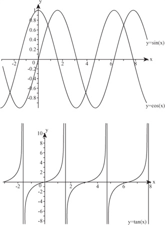
On the bottom of Figure 4.13 is the graph of y = tan(x). The shape of this graph differs from those of the sine waves. One major feature is that a continuous line is not generated. Instead, you see a series of curves with asymptotes every 180°.
The functions sin() and cos() are closely related to circular motion, as is emphasized in Chapter 16. Likewise, their behaviors are surprisingly similar to that of the exp() function. They can be calculated (in radians) by using the following infinite series:

Notice that when x is small, sin(x) is very nearly equal to x. Notice also that sin(0) = 0 and cos(0) = 1.
To extend the basic trigonometric functions, there are also a number of formulas known as the trigonometric identities. The following list states them without proof or even further discussion, but it is a useful exercise to think about how you might prove them. Accordingly, for any value of x and y:

Just as it is important to be able calculate gradients from angles, so it is important to go the other way and calculate angles from gradients. Each of the three trigonometric functions has an inverse function. These are referred to as asin, acos, and atan, abbreviations for arctangent, arccosine, and arcsine. Each inverse function maps from the domain to a range. For all three the domain is [–1, 1]. The sin and cos functions then map to the range [–∞,∞] while the tan function maps to the range [0,360]. Each function takes a number and can map it to more than one angle, so they are multivalued. Still, for each of the functions, there is a standard mapping, as is summarized in the following list.
The inverse of the
sin()function is theasin()function, also expressed asarcsin()and sin-1(). This maps positive values between 0 and 1 to values between 0 and 90°, and negative values greater than or equal to –1 to values between 90° and 180°. For all values of x,arcsin(-x) = 180 -arcsin(x).The inverse of the
cos()function is theacos()function, also expressed asarccos()or cos-1(). This maps values in [0, 1] to the range [0,90°] and values in [–1, 0] to the range [–90°, 0]. For all values of x,arccos(-x) = -arccos(x).The inverse of the
tan()function is theatan(), also expressed as tan-1() orarctan().This maps values in [0,∞] to the range [0, 90°). In the domain [–∞,0] it maps to the range (–90°, 0]. For all values of x,arctan(-x) = -arctan(x).
Note
Domains and ranges are expressed as intervals. Square and curved brackets indicate inclusion and exclusion from intervals. The notation [a, b] indicates the closed interval from a to b, which is the set of real numbers between a and b inclusive. The notation (a, b) in this context means the open interval, the set of real numbers between a and b, not including the numbers a and b. Similarly, [a, b) means the set of numbers greater than or equal to a and less than b.
The inverse trigonometric functions are used in various ways in mathematics, but for programming purposes, used in conjunction with the Pythagorean Theorem, the arctan() function satisfies most of your needs. As becomes evident from an inspection of Figure 4.14, the following two equations show how the ratios given by the hypotenuse and the opposite side (x) of a triangle can be used as arguments to the arctan() function to generate values equal to the inverses of the sin and cos functions.


Because the arctan() function maps infinite quantities to finite ones, it has the unusual ability to cope with fractions with a denominator of zero. Because you can’t use these in programming, it can save time to create a special version of the arctan() function with two arguments instead of one. The two arguments represent the two legs of a right-angled triangle, one of which may be zero. This function is often offered by programming languages as arctan2() or atan2(). Here is how it can be implemented:
function atan2(y, x)
   set deg=1
   if x=0 and y<0 then deg=90
   if x=0 and y>=0 then deg=-90
   if y=0 and x<0 then deg=0
   if y=0 and x>=0 then deg=-180
   if deg=1 then return arctan(y/x)
   otherwise return deg*pi/180
end function
With the help of the trigonometric functions and the Pythagorean Theorem, you can solve problems that involve triangles and more complex figures. This section explores both mathematical and computational aspects of such solutions.
One of the most common challenges to anyone working with triangles is to solve the triangle. Solving a triangle involves using partial information about a triangle to discover all the information, which might include its angles and the lengths of its sides. For example, referring to Figure 4.5, if you are given the triangle ABC and limited information about its angles and sides, using trigonometric functions and the Pythagorean Theorem, it is likely that you can deduce the values concerning sides a, b, c and angles α, β, and γ. To fully solve for a triangle, you seek the following information:
The lengths of the three sides
Any two angles and one side
Any two sides and the angle between them
In a right-angled triangle, the length of any two sides
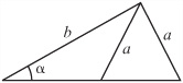
Except for a right-angled triangle, you cannot solve a triangle given two sides and a non-included angle. The reason for this is that there may be two possible triangles, as illustrated in Figure 4.15. Additionally, you cannot solve a triangle if you know only the three angles. The reason is that there are an infinite number of triangles with the same three angles. These angles do not change if the lengths of the sides are proportionately increased or decreased.
The two most powerful methods for solving triangles are called the sine rule and the cosine rule. The sine rule relates angles to the lengths of their opposite sides, while the cosine rule relates one angle to the lengths of the three sides.
The sine rule is particularly neat, and says that for any triangle
To see why this is so, examine the triangle depicted in Figure 4.16. In this figure, a perpendicular line has been dropped from the vertex B to intersect at point P with the line AC. Of such a triangle, you can say that the line BP has length l. Given this start, you can arrive at two equations:
sin(α)=l/c
sin(γ)=l/a
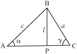
If you rearrange equation 2 and substitute the value of l into equation 1, you get this set of equations:
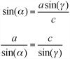
A symmetrical argument applies to b and β.
The cosine rule is a little more complicated, but it is easy to remember because it is an extension of the Pythagorean Theorem. Here is how it reads:
Proving this is a little more involved, but to do so, you can once again use the triangle from Figure 4.16. You’ve denoted the line PC as k units long, making the line AP b – k units (since the whole line is b units). Now you can see from the Pythagorean Theorem that
Eliminating l, you have

You can now eliminate k by using the angle α, since ![]() (from triangle ABP) and k = b – c cos(α). Substituting this value for k, you get
(from triangle ABP) and k = b – c cos(α). Substituting this value for k, you get

Using combinations of these two rules, along with the Pythagorean Theorem and the fact that angles in a triangle sum to 180°, you can solve any solvable triangle. (See Exercise 4.1 for a challenge in this regard.)
As you saw in the previous section, it is possible to have two triangles with the same three angles but sides of different lengths. Two triangles with the same angles are called similar. Since the sum of angles in a triangle is constant, you only need to show that two angles are the same to know the triangles are similar.
The principal fact about similar triangles is that their sides are in the same proportion. As with the rectangles presented in Chapter 2, similar triangles are essentially the same triangle, just drawn to a different scale. This means that if you know two triangles are similar, then you can use the lengths of a side in one to deduce the same measure in the other.
In Figure 4.17, you can see a way to measure the height of a building on a sunny day. Place a stick 1 m long vertically in the ground and measure the length of its shadow. Also measure the length of the shadow of the building. The triangle formed by the tip of the stick T, the base of the stick S, and the end of its shadow U is similar to the triangle formed by the top of the building B, the base of the building A, and the end of its shadow C. The angles at S and A are both right angles, and the angles at U and C are both equal to the angle formed by the sun and the ground. To get exactly the same angle of the sun, you need to align the stick so that U and C are in the same place. The illustration places the two in separate positions to make the basic ideas clearer.

Note
When describing two triangles as similar, you should represent them with the vertices in corresponding order. In other words, if triangles ABC and PQR are similar, the angles at A and P, B and Q, and C and R are the same respectively.
Because the triangles in Figure 4.17 are similar, their sides are in the same proportion. As a result, the ratio of the height of the building AB to the height of the stick ST is equal to the ratio of the length of the building’s shadow AC to the length of the stick’s shadow SU. Expressed in an algebraic form, with the letters in lower case, the ratio is represented like this:
Given this equation, you can calculate c from the values of the other three lengths, all of which you can measure on the ground.
Note
The notation AB for the length of the line from A to B is useful because it means you need fewer symbols in complicated problems. Notice that in this notation, the letters A and B are in normal typeface. When they are written in bold or with an arrow above them (as in ![]() ), they represent not a length but a vector. Vectors are covered in Chapter 5.
), they represent not a length but a vector. Vectors are covered in Chapter 5.
If two triangles have sides of the same lengths and angles of the same size, then they are said to be congruent, which means that they are exactly the same or at most mirror images of one another. While congruence is often used in the area of geometrical proofs, it seldom appears in programming problems.
Depending on which measurements you know, there are various ways to measure the area of a triangle. You can use the triangle depicted in Figure 4.16 again to derive one method. Using this method, you take a triangle ABC and drop a perpendicular of length l from the vertex B to the point P on the line AC. This divides the triangle into two right-angled triangles.
Then you draw congruent right-angled triangles alongside each of these to create two adjacent rectangles, each of which is twice the area of the corresponding right-angled triangle. The total area of this rectangle is twice the area of the triangle ABC, so you say that the area of a triangle is ![]() (base × height).
(base × height).
You can also find the area knowing other measurements. For example, if you look at the triangle ACP, you can see that l = b sin (γ), so you can substitute this value into the previous formula to get the area as ![]() ab sin(γ).
ab sin(γ).
In programming you most commonly use the trigonometric functions when working with objects that need to rotate. The final sections of this chapter examine the relationships between the trigonometric functions and rotation.
An object drawn on the computer screen could be described in terms of the positions of its vertices. In Figure 4.18, you see one triangle (T) represented in different positions on a monitor screen. Recall that, as previously mentioned, the (0, 0) coordinate of the y-axis is in the upper left of the screen. Accordingly, triangle T initially has vertices at (100, 150), (125, 125) and (150, 130). Given this start, there are then a number of different ways you can move this triangle to a new position. Each of these is called a transformation.
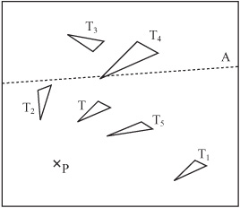
With reference to Figure 4.18, here are some of the ways that triangle T can be transformed:
Translation. If you move the figure to a new position without rotating it (as with triangle T1), the change is called a translation. A translation is described by a vector, which is a topic examined Chapter 5. For the moment, just think of it as a value describing how far you are moving the figure in the x and y directions.
Rotation. If you turn the figure around by an angle (see triangle T2), the change is called a rotation. A rotation is described by a single point and an angle. You say that triangle T2 is the result of “rotating triangle T by 45° about the point P.” The single point of rotation is sometimes called the center of rotation. The angle is called the angle of rotation and is usually measured clockwise on a graph or counter-clockwise on a computer.
Reflection. If you flip the figure over (see triangle T3), the change is a reflection. A reflection is defined by a single line known as the axis of reflection. You say that triangle T3 is the result of “reflecting triangle T in the axis A (the line y = x).”
Scaling. If you change the size of the figure (see triangle T4), the change is a scale. Scaling an object can be defined by a single point and a number representing the proportion of the size of the new figure to the old one. The single point is the origin of the scaled object and should not be confused with the origin of a graph. The number representing proportion is called the scale factor. Given these specifics, T4 is the result of “scaling T by a factor of 1.5 from the point P.” You can also perform more complex scaling by scaling different portions of the object in particular directions.
Shearing. If you take hold of one point of a triangle and shift it across relative to the others, you shear the triangle (see triangle T5). Shearing is defined in terms of a single line (the line of invariance) and a number representing the amount of shearing (the shear factor).
Each of these transformations can be calculated numerically by performing various operations on the vertices of the object. Many of these calculations involve the trigonometric functions explored in the previous sections.
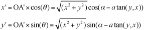
Figure 4.19 represents triangle T (ABC). This triangle is to be rotated by an angle α around the origin O to make a new triangle T’ (A’B’C’). To accomplish this, you use the y-axis, and as mentioned previously, with respect to monitor coordinates, it is measured downward. To represent the rotation, lines are drawn from the origin O to the points A = (x,y) and A’ = (x’, y’). Also lines are drawn from A and A’ to the x- and y-axes and the points X, X’, Y, and Y’, where these lines meet the axes.

Additionally, the lines OX and OY have lengths x and y, respectively, while the lines for OX’ and OY’ have lengths x’ and y’. Further, the lengths of OA and OA’ are both the same (as this is a defining feature of a rotation).
What can you deduce from all this information? Well, first you know that since OA = OA’, using the Pythagorean Theorem, you can say that ![]() . Second, you can calculate the value of the angle between OA and the x-axis (called θ in the diagram) as
. Second, you can calculate the value of the angle between OA and the x-axis (called θ in the diagram) as atan(y, x).
Because the angle of rotation is α, you know that the angle θ’, between OA’ and the x-axis, is equal to α–θ = α – atan (x, y). This means you can calculate the value of x’ and y’ as follows:
Repeating the operation for each of the vertices of the triangle rotates the whole triangle about the origin.
Note
When calculating x’ and y’, you need to be careful about the signs of x and y. Since it ensures that the correct value of the angle is returned, it is best to use the two-argument implementation of atan(), atan(y, x), in functions like these.
What if you want to rotate the object around a point other than the origin? To accomplish this, you can use a trick. First, you translate the object so that the center of rotation lies on the origin. Then you rotate it and translate it back. This approach to the problem is based on the idea of a vector. (Again, this will be covered in Chapter 5.)
To rotate a point (x, y) by an angle α around the point P = (s, t), first you translate it by subtracting (s, t) from each point. Then you rotate by α around the origin. Finally you add (s, t) to the resultant points. This gives a complicated formula for the values of x’ and y’:
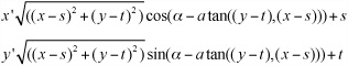
You can see the relationship of these formulas to those you saw before. Each one is a result of replacing x and y with x – s and y – t, respectively, and then adding s or t as appropriate. Combining transformations in this way provides a powerful tool that you will see much more of in later chapters.
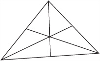
When programming the movements of graphical objects, you often want to rotate an object around its own center. The center of an object is often called the center of gravity or center of mass. This is especially the case if you are working with a three-dimensional object. For a triangle in two dimensions, this point is called the centrum. As illustrated by Figure 4.20, the centrum is found at the intersection of the three lines joining the vertices to the midpoints of the opposite sides.
To find the centrum, you find the mean of the three vertices. To accomplish this, consider that if the vertices are at (x1, y1), (x2, y2) and (x3, y3), the centrum is at the point ![]() . Discovering the centrum is a challenge presented in Exercise 4.2.
. Discovering the centrum is a challenge presented in Exercise 4.2.
Note
The arithmetic mean (or just mean) of a number of values a1,a2,...,an is the sum of the values divided by the number of values: ![]() . This may be written using the notation
. This may be written using the notation ![]() , where the capital Greek letter sigma (∑) denotes a sum of values over the index i. The mean is often referred to as the average, but mathematicians use the word average to mean a number of different functions. These include the arithmetic mean, the geometric mean, harmonic mean, median, and mode, each of which is useful in different circumstances.
, where the capital Greek letter sigma (∑) denotes a sum of values over the index i. The mean is often referred to as the average, but mathematicians use the word average to mean a number of different functions. These include the arithmetic mean, the geometric mean, harmonic mean, median, and mode, each of which is useful in different circumstances.
While it is useful to be able to rotate an object about any axis, it is also handy to know a few shortcuts. Rotating by certain common angles is much simpler. Here are a few shortcuts commonly used:
To rotate the point (x, y) by 180° about the origin, multiply both coordinates by –1, getting (–x, –y).
To rotate (x, y) by 90° about the origin, switch the coordinates around to get (y, –x).
To rotate (x, y) by –90° about the origin, switch the coordinates the other way to get (–y, x).
These operations can be derived from equations given previously in this chapter.
As you have seen in previous sections of this chapter, a reflection can be specified by giving a single line on the plane. This line is called the axis of reflection. As illustrated by Figure 4.21, the image of a point P reflected in a particular axis A is the point P’ such that two conditions are met. First AP = AP’. Second the line PP’ is perpendicular to A.
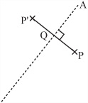
Although you can calculate the position of P’ from this information, it is hard to do so without vectors. However, you can also use rotations and translations to reduce this to a simpler problem. Reflecting in the x- or y-axis is very simple. Accordingly, the point (x, y) reflected in the x-axis gives the point (x, –y), and in the y-axis it gives (–x, y). Therefore, to reflect P = (x, y) in an axis with the equation y = mx + c, you can do the following, as is illustrated by Figure 4.22:
Translate P by –c units in the y direction to get P1 =(x, y–c) = (x1, y1).
Rotate P1 by atan(m) about the origin to get
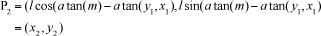
where
 is the length of the line OP’.
Reflect P2 in the x-axis to get P2 = (x2, –y2) = (x3, y3).
Rotate P3 by –atan(m) about the origin to get

Translate P4 by c units in the y direction to get P’ = (x4, y4 + c) = (x’, y’).

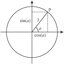
The trigonometric functions are not just mathematical abstractions introduced to make calculations easier. They represent a common phenomenon. Imagine that you have a point P at a distance of 1 unit from the origin, as is shown in Figure 4.23. As you can see from the definition of the sin() and cos() functions, the coordinates of P must be (cos(a),sin(a)), where a is the angle the line OP makes with the x-axis. If you plot all such points P, you make a circle around the origin.
Note
Notice that the length of the line OP is 1. This proves the identity you saw earlier, which established that sin2θ + cos2θ = 1.
To draw a circle using the sin() and cos() functions, you represent the positions of a point moving around a circle at a constant speed. Assuming it starts horizontally, if you were to drive a pin into the side of a wheel, the vertical position of the wheel over time as the wheel spins expresses the output of the sin() function. Chapter 16, which covers oscillations, provides further discussion of this topic. For now, simply note that any point on a circle with radius r centered on the point (x, y) has coordinates (rsin(α), rcos(α)) for some value of α.
Write a function solvetnangle(tnangle) that takes an array representing a triangle with incomplete information and returns the array filled in as far as possible.
Your function should accept a six-element array in which the first three elements are the lengths of the sides and the last three are angles. The angles may be in degrees or radians, depending on your preference. Any of these values may be replaced with the string “?” representing an unknown. The function should return 0 if the triangle is impossible, a complete array of six numbers if the triangle can be solved, and an incomplete array if it cannot be solved uniquely.
Write a function rotatetofollow(triangle,point) that rotates a particular triangle around its centrum to aim at a given point.
The function should take two arguments, one array representing the three vertices of the triangle (the first of which is taken to be the “front”), another giving the point to aim at. It should return the new vertices of the triangle. If you have trouble with this exercise, you might want to come back to it after reading the next chapter.
In this chapter, you have begun to explore the world of geometry, and you have already learned a number of vital techniques that are useful in animation and games. In the next chapter, you will fill in a lot of the blanks left by this chapter.
The meaning of angle and the different ways that an angle can be measured
The meaning of the term area and how to measure the areas of arbitrary rectangles, circles, or triangles
The various types of triangles—scalene, isosceles, equilateral, right-angled—and their properties
How to use the trigonometric functions and the Pythagorean Theorem to solve problems in right-angled and other triangles
The meaning of the terms similar and congruent and what they imply for lengths and angles of shapes
The meanings of rotation, reflection, translation, scale, and shear, and how to calculate the first three of these for a given point or shape on the plane