The tension in a spring can be calculated very simply. To describe how stretchy it is, a spring has a value called the coefficient of elasticity, k. The tension in a stretched spring is then proportional to its extension, and the extension is the difference between its current length and its length when it is not stretched. The value of this difference is given by Hooke’s law:

Why the negative sign? This is conventional because the force is always directed backward, toward the unstretched “equilibrium” length. As shown in Figure 16.1, if a particle is attached to the end of the spring, it experiences the tension backward along the length of the spring.

Figure 16.1. A particle on the end of a spring.

Some springs are only extensive. In other words, they experience a tension only when stretched outward. While an extensive spring becomes something more like a rigid rod, an elastic band has no tension when unstretched. Other springs are compressive. Compressive springs experience a tension outward when their length is less than the standard length. One generalization you can draw from observing extensive and compressive springs is that a negative extension leads to a positive tension.

When a spring is under tension (compressive or extensive), it contains energy, known as elastic potential energy. It takes work to stretch a spring, and the energy is released when it is allowed to bounce back. The energy is given by

From this and the equation for force, you can see that the coefficient of elasticity has units of kg s^–2.

There is one other facet of real-life springs that is important to consider. Real-life springs cannot be stretched indefinitely. Instead, they reach a length called the elastic limit. Beyond this point, the coefficient of elasticity increases significantly, making them much harder to stretch. In addition, after they have reached their elastic limit, springs will no longer return to their original length when released. At an extreme, springs can be stretched to the point that even the bonds between their constituent molecules start to break. At this point, the springs are likely to snap. For the current context of discussion, you can simply say that beyond the elastic limit, springs start to act like inextensible strings, with constant inward tensions.

Figure 16.2 illustrates the canonical example of springs in action. Here, you have an object with mass m attached to one end of an extensive spring with unstretched length l. The other end of the spring is attached to a supporting beam or the ceiling.

Figure 16.2. A particle hanging from a spring.

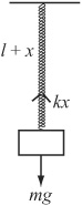
If the object hanging on the spring is in equilibrium, you can say that the tension in the spring must be equal to its weight. This is expressed as follows:

Since for a particular spring in constant gravity the values of g and k are constant, the extension of a spring is directly proportional to the mass of the object hanging on the spring. For this reason, you can use a spring to measure something’s weight.

If the object is somewhere other than in the equilibrium position, with an arbitrary extension x, then the force on it is equal to mg – kx. This difference describes a different situation. In this situation, the object is moving horizontally under the action of a spring that is both compressive and extensive. The unstretched length of this spring is given by the expression , the equilibrium length of the first spring. This value is useful since it allows you to ignore gravity when calculating the motion of the object attached to the spring.

To calculate the equation for simple harmonic motion, you can begin by looking at the formula for Hooke’s law. By applying Newton’s second law, you see that

where x is the extension, m is the mass, and a is the acceleration. All of these quantities must be measured in the same direction. Here is another version, given as a differential equation:

As you have seen (in Chapter 6 and elsewhere), differential equations require a great deal of work. In this case, it turns out that a simple function solves it. You’ve already encountered two functions whose second derivative is their own negative. These are sin() and cos(). Given these two functions, recall that

It takes only a little tweaking to adapt these functions to create a general formula that solves the differential equation for SHM:

where A and B, are arbitrary constants and ωis equal to . Another useful way of presenting this relationship is as follows:

where C and p are arbitrary constants. You’ll be using this form of the equation here, although both forms are common.

You can calculate the velocity of the object attached to a string at a particular time by differentiating the SHM equation, which gives you

Differentiating again gives you

as required.

As usual with a differential equation, you have a family of equations that all serve as valid solutions. Any one of these provides a possible motion for the object on the spring. By setting the initial condition, you choose which to use. In other words, you choose what the object is doing at the start. If you pull it down by a certain distance d and then release it, then you will get C = d, p = 0. If you give the object on the spring a push from equilibrium, so that it has an initial velocity v, you get . You’ll look at these calculations more in a moment.

So what does all this mean? What does the motion look like? One answer is that when , since sin(0) = 0 and cos(0) = 1, the particle has the position 0 and velocity Cω If C is positive, the extension gradually increases, until at time , when it reaches a maximum of C. Then it decreases to 0 again and goes back the other way, before returning to 0 at .

As shown in Figure 16.3, the result of this action is the generic sine wave discussed in Chapter 4. The time is called the period of the motion. The period of the motion is the time required for one complete oscillation. The value ωis called the frequency. The value p is called the phase of the motion. The phase of the motion is how far the waveform is shifted from zero along the time axis. And C is called the amplitude, or maximum displacement from equilibrium.

Figure 16.3. The position of a particle over time under SHM.

As you might recall, the position of a particle when moving along a sine wave is equivalent to the y-coordinate of a point on the circumference of a turning wheel. This means that a point on a wheel moves under SHM. In fact, as Figure 16.4 illustrates, the values C and p relate to this interpretation. C is the radius of the wheel, and p is a measure of how far around the wheel the object is located or has traveled.

Figure 16.4. SHM and circular motion.

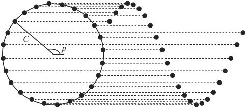
You take advantage of this when using circular motion to drive pistons. When you attach a rod to a point on a wheel and allow it to slide up and down as the wheel turns, its tip approximately oscillates under SHM.

SHM also occurs in the motion of a pendulum. Again, it is an approximation and only works when the oscillations are small. When an object is attached to a pendulum by a light inextensible string of length l at an angle θ, it experiences a force W downward due to its weight and a tension T from the string. In particular, the radial force on the object (which provides torque) is –W sin θ The minus sign is used to indicate that the force is directed in the opposite direction to the angle. As noted before, for small values of θ—oscillations of about 5°—sinθ is very close to θ so the torque acting on the particle is approximately –Wlθ. This gives you another example of Hooke’s law:

In this case, the mass of the particle cancels out, and the frequency depends only on the length of the string. Consequently, the period is proportional to the square root of the length.

Other examples of SHM in action include a buoy floating on wavy water, the vibration of a plucked guitar string, the vibrations of atoms in a crystal, the variation of an alternating current, and the variation in a population of animals over time. Whenever you find a situation where there is an equilibrium position and a force that is exerted continuously to try to restore that equilibrium, you will find SHM.

It’s also worth noting that waves themselves are formed of components moving under SHM. A light wave consists of oscillating electric and magnetic fields. The strength of these fields at any particular location varies over time in an SHM pattern. Each oscillation induces an oscillation next to it, and the next oscillation lags a little behind. The result is that the situation looks like a sine wave traveling forward over time. This phenomenon will be examined further later in the chapter.

To return to the question of the parameters C and p, as was discussed previously, C represents amplitude and p represents phase of the motion, respectively. While a particular mass on a particular spring will always oscillate with the same frequency, the amplitude and phase vary from situation to situation, according to how fast the particle is put into motion and how far away from equilibrium it is released.

The easiest way to calculate these values is to know the velocity v and extension d at time 0. To determine the parameter values, you can use the velocity and position formulae of SHM as simultaneous equations:

so

which is to say,

More generally, you can do the same calculations for any time t: the calculation for C remains unchanged while the calculation for p merely changes to

Damped harmonic motion (DHM) is a slight modification to the SHM equation. You add a new damping factor to the differential equation. This factor is proportional to the velocity rather than the acceleration:

Solving this differential equation is a little more work than before. It involves using a “trial solution,” which leads to a particular quadratic equation. Leaving out the details, the end result is as follows:

where

Depending on the values of D and ω this equation renders different results. If you define the variable αto be D² – ω², if α > 0, this equation has real solutions, and you end up with a family of equations of the form

When α = 0, so that D = ω while the motion is similar to what has been previously described, only one value of r occurs. The result is that you get a slightly simpler equation:

If α < 0, then the equation has no real roots, and you end up with a complex number. This is not the place to discuss complex numbers, but it turns out that you can still solve the resulting differential equation by using the imaginary number i. This number, by definition, equals the square root of –1. Using this approach, you can derive this formula:

where

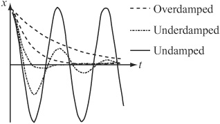
While harder to discover, this equation resembles the SHM equation discussed previously, but there are two main differences. The first is that it has the additional exponential term, which is negative. As a result of this, the amplitude of the motion decreases over time. The second is that the frequency is different. The greater the value of D, the lower the frequency. This continues until D reaches the critical damping value where D=ω Above that value, you go into the first kind of behavior, and the frequency is essentially zero. In other words, rather than oscillating, the object follows an exponential curve. In sum, then, there are three “zones” of behavior for DHM:

Figure 16.5 illustrates the different behaviors of these three forms of damping.

Figure 16.5. Possible motions of a particle under different levels of damping. Each starts with the same initial conditions, and all the springs have the same coefficient of elasticity.

As was done with previous equations, you can differentiate each of the motion formulas to get the velocity function.

For underdamping, you arrive at the following:

For critical damping, the result is as follows:

(Remember that for critical damping, D = ω).

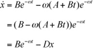
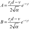
And for overdamping, you get this result:

Expressed more simply, differentiating overdamping appears this way:

Applying damping involves little more than plugging values into these equations. But calculating the parameters is more detailed than before because the velocity function is more complicated.

When you work with the equations, recall that D is a known constant property of the spring, like the coefficient of elasticity, not a parameter like C and p. If you know the distance and velocity at time t as before, then you can work with them through a sequence of equations.

To start with, for underdamping, you have

so

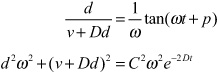
and this gives you

With critical damping, you have this formulation:

so

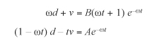
If t = 0, then working with critical damping becomes even simpler:

As for overdamping, you have:

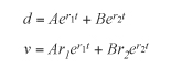
so

and this gives you

Again, if t = 0, you can use a simpler formulation:

Everyone has heard stories about people who can use their voices to break glass. This isn’t just a matter of producing particularly high notes that miraculously cause things to break. A physical phenomenon is behind it that is a major consequence of SHM.

Imagine a simple variation in the situation represented by Figure 16.2. This time, the top of the spring is attached to a vibrating rod. The vibrating rod moves it up and down at a certain driving frequency f with an amplitude of A. As becomes apparent after a brief discussion, the driving oscillation imparts a force to the system. Each time the bar moves up, it increases the tension in the spring. When it drops, it releases it. What then happens to the object suspended from the spring?

To answer this question, while the object bounces around rather erratically, some patterns emerge. In particular, if you change the driving frequency, the amplitude of the motion of the object increases as you get closer to the natural frequency of the spring. When you reach the natural frequency, the particle starts to go crazy. It bounces higher and higher without end. In fact, theoretically, it might bounce infinitely high. Then as you increase the driving frequency further, the particle calms down again.

There’s a reasonably simple relationship between the amplitude C of the motion and the driving frequency. This relationship can be expressed as follows:

Here the value kA represents the maximum force exerted by the driving oscillation—the driving force.

When the driving frequency is equal to the natural frequency ωthe first term in the square root drops out. In SHM, with D = 0, this means that C becomes infinitely large. Otherwise, C is inversely proportional to the damping factor. As a result, in systems with little or no damping, the oscillation starts to spiral out of control. Such spiraling is called resonance, and the natural frequency is called the resonant frequency.

You use this principle every time you push a child on a swing. At the topmost point of the swing, you apply a force. This force is naturally applied at the same frequency as the oscillation, with the result that the oscillation grows in amplitude and fun. Because a pane of glass also has a natural frequency, if you drive it with a sound wave of the same frequency, it vibrates so hard that it shatters.

All of this shows that when you create a spring system in a simulation, it’s important to give it some damping factor, or at least an elastic limit. Otherwise, you might find things getting out of hand.

When you combine two springs together by means of another, the combined springs are said to be coupled. Coupling means that the motion of each spring is affected by the other. Energy is constantly being transferred between them. The result is that extremely complicated motion can result. There’s no need to look into the mathematics in detail, but it’s worth noting one particular result.

If two identical coupled springs are set in motion in the same phase, then they will swing in parallel at the natural frequency. This is true despite the fact that both are experiencing a tension due to the coupling spring. If they are set in motion exactly out of phase, meaning that one is lifted up as the other is pulled down and then they are both released at the same time, they will continue to oscillate out of phase. However, the frequency will be higher than before. These are called the two natural modes of the motion.

In general, any two coupled oscillators yield a system with two natural modes, each with its own frequency. The modes depend on the frequencies of the two oscillators and of the coupling spring. Any other motion of the system is actually a linear sum of two such oscillations. These concepts are very important in acoustics.

The three functions are useful in different circumstances. The first is a pure mechanical system. With such a system, the function returns the force on the object on the spring due to the spring. In this case, you must need to apply gravity separately. This is the only method you can use in general circumstances, such as when neither end point of the spring is fixed in place. Here is the forceDueToSpring() function:

function forceDueToSpring(end1, end2, velocity1,
                          velocity2, springLength, elasticity,
                          damping, elasticLimit,
                          compressiveness, minLength)
  // The object you're interested in is attached to end2
  set v to end1-end2
  set d to magnitude(v)
  if d=0 then return vector(0,0)
   // skip for this time-step if they coincide

// loose elastics have no force when compressed
  if d<=springLength then
    if compressiveness="loose" then return vector(0,0)
  end if

  // apply second elastic limit (inextensible behavior)
  if d>=elasticLimit*1.2 or d<=minLength*0.9
                           or (d<=springLength*0.9
                           and compressiveness="rigid") then
    return "bounce"
  end if

  // apply first elastic limit (increased force and damping)
  if d>=elasticLimit or d<=minLength
                       or (d<=springLength
                       and compressiveness=#rigid) then
    multiply elasticity by 20
    set damping to max(damping*10,20)
  end if

  // calculate force by Hooke's law
  set e to d-springLength
  set v to v/d
  if damping>0 then
    set vel to component(velocity1-velocity2,v)
    set f to damping*vel+elasticity*e
  else
    set f to elasticity*e
  end if
  return f*v
end function

The only complicated part of the forceDueToSpring() function involves dealing with the elastic limit. Simulated springs are more complicated than real ones because you can get impossible situations, like a spring that is extended significantly beyond its elastic limit. This happens both by incorrectly setting up the simulation. This can happen if users are allowed to drag objects around. Such situations can be avoided. On the other hand, other problems arise, such as when resonance is coupled with a gradual accumulation of rounding errors.

To deal with this, you can create a tiered elastic limit system. Beyond the set elastic limit of the spring, you increase both the coefficient of elasticity and the damping coefficient. The effect of increasing the coefficient of elasticity is to create a strong force inward, which is important. But the damping coefficient is also necessary because it ensures that the system loses energy rapidly, which means that on the next oscillation it doesn’t exceed the elastic limit.

You also create a second elastic limit, arbitrarily set at 1.2 times the first. If the spring is trying to extend beyond this point, you treat it as a collision with a solid wall perpendicular to the spring. This ensures that the spring can never extend past the second limit.

The second method is designed for situations that are slightly simpler than those typical of the previous section. These situations often involve undamped, uncoupled springs. With such springs, the spring attaches a movable object to a fixed point. The object can move freely in all directions. For example, this method would be suitable for situations where a user can click and throw the object, or where the object is part of a system with collisions. In these cases, you can take advantage of conservation of energy to avoid the inevitable rounding errors that appear when dealing with forces applied individually at each time step. By knowing that the total energy of the particle is constant, you can calculate its speed at any moment as long as you know its position. The system can even deal with the situation when the “fixed” point is in fact moving under the user’s control. The particleOnSpring() function addresses undamped and uncoupled springs.

function particleOnSpring (end1, end2, speed,
                           direction, mass, totalEnergy,
                           springLength, elasticity,
                           compressive, timeStep, g)
  // Returns a list of position, speed, direction, and total energy.
  // totalEnergy can have the value "unknown",
  //in which case the function calculates it and returns it.

  set v to end1-end2
  set d to mag(v)
  set e to d-springLength

  if totalEnergy="unknown" then
    // calculate energy
    set totalEnergy to mass*speed*speed/2
    if e>0 or compressive=TRUE then
      set epe to elasticity*e*e/2
      add epe to totalEnergy
    end if
    if g>0 then
      set gpe to mass*g*end2[2]
      subtract gpe from totalEnergy
    end if
  end if

  // calculate force
  set f to vector(0,mass*g)
  if e>0 or compressive=TRUE then
    if d>0 then
      add v*elasticity*e/d to f
    end if

  end if

  // calculate new position
  set a to f/mass
  set displacement to direction*speed*timeStep + a*timeStep*timeStep/2
  set pos to end2 + displacement

  // calculate new elastic energy
  set newd to mag(pos-end1)
  set newe to newd-springLength
  if newe>0 or compressive=TRUE then
    set epe to elasticity*newe*newe/2
  otherwise
    set epe to 0
  end if

  // calculate new kinetic energy and hence speed
  set ke to totalEnergy-epe+mass*g*pos[2]
  if ke<=0 then // NB: for safety
    set speed to 0
  otherwise
    set speed to sqrt(2*ke/mass)
    set velocity to norm(displacement)
  end if

  return Array(pos,speed,velocity,totalEnergy)
end function

Your final function is the simplest. It addresses pure damped harmonic motion oscillation (or SHM if damping = 0). Feed it an initial position and velocity and a time t, and it calculates the position and velocity at that time. This calculation is performed through a set of three functions. The primary function is the calculateDHMparameters() function. Since it is wasteful to calculate the parameters more than once, the best approach is to store them. The first function calculates the parameters and the form of the motion. The other two calculate the actual values when fed with the results of the first.

function calculateDHMparameters(initialPos, initialVel,
                                    elasticity, damping)
   set omega to sqrt(elasticity)
   set d to damping/2
   set alpha to elasticity-d*d
   if d=0 then
      set p to atan(omega*initialPos/initialVel)
      set c to sqrt(elasticity * initialPos *
                     initialPos + initialVel * initialVel)/omega
      return array("SHM", p, c)
   else if d<omega then
      set v to initialVel + d * initialPos
      set p to atan(initialPos * omega / v)
      set s to initialPos * initialPos * elasticity + v * v
      set c to sqrt(s)/omega
      return array("UnderDamped", p, c, sqrt(-alpha))
   else if d=omega then
      return array("Critical", initialPos, omega *
                     initialPos + initialVel)

   else
      set sq to sqrt(alpha)
      set r1 to -d-sq
      set r2 to -d+sq
      set a to (r2*initialPos - initialVel)/(2*sq)
      set b to -(r1*initialPos - initialVel)/(2*sq)
      return array("OverDamped", a, b, rl, r2)
   end if
end function

Given use of the calculateDHMparameters() function, you then call the get OscillatorPosition() function, which is defined as follows:

function getOscillatorPosition (elasticity, damping, params, time)
   set omega to sqrt(elasticity)
   set d to damping/2

   if params[1] is
      "SHM": return params[3] * sin(omega * time + params[2])
      "UnderDamped": return params[3] *
           sin(params[4] * time + params[2]) * exp(-d * time)
      "Critical": return (params[2] + time * params[3]) * exp(-d*time)
      "OverDamped": return params[2] * exp(params[4]*time +
                     params[3] * exp(params[5]*time)
   end if
end function

Having called both the calculateDHMparameters() function and the getOscillator Position() function, you can then call the getOscillatorSpeed() function. This function is defined as follows:

function getOscillatorSpeed(elasticity, damping, params, time, pos)
   // determine pos before running this function
   set omega to sqrt(elasticity)
   set d to damping/2

   if params[1] is
      "SHM": return params[3] * omega * cos(omega *
                     time + params[2])
      "UnderDamped": return params[3] * omega * cos(params[4] *
                              time + params[2]) * exp(-d * time) - d*pos

      "Critical": return params[3] * exp(-d*time) - d*pos
      "OverDamped": return params[2] * params[4] *
                                         exp(params[4]*time] + params[3] *
                                         params[5] * exp(params[5]*time)
   end if
end function

All three of these functions represent little more than the application of the equations shown previously for SHM and DHM. It is important, however, to notice that the variables used to pass the values from function to function are global, so the three are interdependent.

A wave is a set of individual coupled oscillators. Each performs some oscillation and so induces an oscillation further down the line, slightly out of phase with the previous oscillation. Showing the oscillations at a frozen moment in time, Figure 16.6 illustrates the result.

Figure 16.6. A series of coupled oscillations

As you can see in Figure 16.6, the silhouette of this picture is a sine wave. As it is, the shape of the wave does not always follow a sine pattern, but whatever the shape, the oscillations are copies of the driving oscillation at one end of the wave.

That waves are generated by a driving oscillation gives rise to a second way of picturing a wave. According to this view, the wave is a moving waveform. A waveform is an object moving at a certain velocity. To describe the waveform as an object is not quite accurate, however. Rather than an object, it is a kind of virtual object. It is a packet of energy transmitted through some medium.

Given the view provided by the waveform, the velocity of a wave is the distance traveled over time by the waveform. This value is determined by the physical properties of the medium. For a sine wave, you can measure the position of successive wavefronts over time. A wavefront is a peak of the waveform.

Once you know the speed v of the wave and its frequency f, you can calculate the distance between successive wavefronts. This value is referred to as the wavelength, denoted λ. This gives you a simple equation relating the three quantities: v=fλ

There are two principal kinds of wave, transverse and longitudinal. A transverse wave is the kind pictured in Figure 16.6. With a transverse wave, the oscillators are aligned perpendicularly to the direction of travel of the wave. Among such waves are water waves and electromagnetic waves. Electromagnetic waves are also known as light.

Longitudinal waves are a little harder to picture. The simplest example is a coiled spring (such as a Slinky, the children’s toy). When the string is stretched out and a sudden push is given to one end, a ripple travels through the coils. Each coil vibrates forward and backward along the direction of motion of the ripple.

Another type of sound wave, as illustrated in Figure 16.7, is caused by air molecules vibrating backward and forward, creating small areas of lower and higher pressures. The low and high areas tend to restore equilibrium. Low areas are referred to as rarefaction. High areas are referred to as compressions.

Figure 16.7. A longitudinal wave.

Although they have different physical causes, the transverse and longitudinal waves behave in essentially the same way. You often display longitudinal waves by a graph of pressure against time, which looks exactly like any other waveform. Longitudinal waves also reflect, refract, and diffuse exactly as transverse waves do.

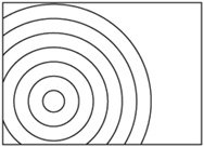
As shown in Figure 16.8, both types of wave are often also drawn in a kind of “plan view,” where the wave is represented by a series of lines representing particular wavefronts.

Figure 16.8. A wave represented as a succession of wavefronts.

Because a wave is a virtual object, it’s perfectly possible for several waves to be traveling through the same medium. In fact, this happens routinely. The air around you, for example, contains what could be considered to be an infinite number of different waves of light traveling in all directions. However, because waves are virtual, it’s only humans who consider this to be happening. In reality, all that is going on is a constant fluctuation of electromagnetic fields in space. The fact that energy is being transferred in the process is almost accidental.

You can conceive of waves in these two contradictory ways because they have an important property. They can be combined together into a single, more complex wave. For example, you can combine the two waves in Figure 16.9 into a single, more complex waveform just by adding the displacement values at each point.

Figure 16.9. Adding waves.

Combining waves creates some interesting effects. Among other things, if you add two waves together that are exactly out of phase, they combine to give a straight line. No wave at all results. Three waves, all mutually out of phase by 2π/3, produce the same result. Drawing on this occurrence, in order to decrease the total current flow, electricity is often transmitted in three simultaneous waves out of phase with one another.

If you can combine waves, you can also decompose a wave into others by subtracting them. A technique called Fourier analysis allows you to decompose any waveform, no matter how complex, into sine waves of varying amplitude and phase. This is essentially what you do when listening to sound. You try to separate out different waveforms that correspond to different sound sources.

The result of decomposing a wave into individual sine waves is the spectrum of the wave. The spectrum of the wave is a kind of “signature” for a particular wave emitter. The plural of spectrum is spectra, and spectra are used in many contexts for different types of analysis. In one application, they are used to distinguish different kinds of chemical elements. When burned, each element emits a characteristic spectrum of light radiation. This allows you to work out the chemical composition of distant stars, and to find out some other interesting facts.

In contrast to light, particular musical instruments also have a characteristic sound spectrum (timbre), consisting of different integer and fraction multiples of the primary note. A sound wave is perceived as a particular note according to the frequency. Your perception of a complex waveform as a single sound at a single frequency is a very impressive bit of mental computation, and is the equivalent to your perception of a complex spectrum of light wavelengths as a single color. This topic is addressed once again in Chapter 20.

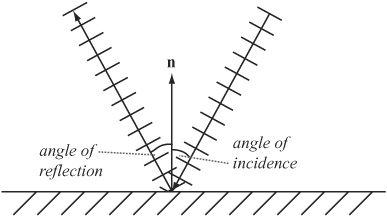
Several important behaviors of waves are a consequence of their physics. Consider first reflection. When a wave strikes a barrier of some kind, depending on the natures of the wave and the barrier it encounters, it reflects off the barrier. If the barrier can’t absorb the energy, the wave is sent back to where it came from. As Figure 16.10 illustrates, the wave reacts exactly like an elastic collision, bouncing off the wall at the same angle as it is struck. The angle at which the wave strikes the wall is the angle of incidence. The angle at which it bounces off the wall is the angle of reflection.

Figure 16.10. Reflection.

A further form of behavior typical of waves is called refraction. Refraction occurs when the velocity of the wave changes. If you imagine a line of cars traveling at a speed of 60 mph hitting a zone where it has to travel at 30 mph, you can see that in the slower zone, the cars will end up bunched closer together. The same thing happens to the wavefronts of a wave. As the wave hits a new medium where its velocity is lower, the wavelength has to decrease. This can also be seen directly from the wave equation. The frequency of the wave is being generated somewhere else, and since the frequency of the wave depends only on the driving oscillation, it is fixed for any particular wave.

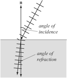
Changing the wavelength has other consequences, as is illustrated in Figure 16.11. When a succession of wavefronts hits a new medium at an angle, certain parts of the wave hit the start of the new medium (called the interface) earlier than others. This causes the wave to change its direction, like steering a tractor or tank by altering the relative speeds of the two tracks.

Figure 16.11. Refraction.

You see this effect whenever you look at a straw in a glass of water. At the point at which it enters the water, the straw appears to be broken. The appearance of the straw is further complicated by the fact that different wavelengths travel at different speeds in the water. The result is that the waves change directions by different amounts. A wave made up of several different wavelengths will split into a fan of rays, creating a prism effect as seen with rainbows. The amount by which a particular wave is deflected is described by Snell’s law, which says that if α is the angle of incidence and β is the angle of refraction, they are related by

where the n values are constant properties of the media through which the wave is traveling, called the index of refraction. For light, this value is equal to the quotient of the speed of light in a vacuum, c, with the speed of this wavelength in the medium.

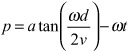
Another phenomenon is called the Doppler effect. To understand how this works, consider the images of Heathcliff and Cathy. Suppose Heathcliff is traveling past Cathy on a train and calls out to her. The speed of the train causes the wavelength of the sound, as Cathy hears it, to shorten. This is so because, as Heathcliff travels forward, each wavefront is emitted closer to the previous one.

You can also calculate the Doppler shift. The Doppler shift is the amount by which the wavelength is shifted. If the train has a speed s and the sound has a frequency f, then the wavelength will be decreased by a value . If this takes the wavelength to a value less than zero, however, you’ll hit a problem. This occurs when s is equal to the speed of sound, approximately 330 m/s. At this point, the wave is overtaken by the wave emitter, and you get a sonic boom. The calculation works equally well as Heathcliff disappears into the sunset. In this case, you use a negative speed for s. If Cathy is somewhere over the hills from the train, then you’ll need to use the dot product to find the component of the train’s velocity that’s traveling in her direction.

The Doppler effect is used as one of the principal pieces of evidence for the expansion of the universe. As mentioned earlier, the characteristic spectrum of elements is used to determine the composition of stars. When you examine these spectra for particular stars, you find that on average they are all red-shifted. In other words, their wavelengths have increased because the stars are moving away from you. What’s more, the rate at which they are moving away depends on their distance from you, and this suggests a picture of the universe as constantly expanding from an explosion.

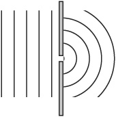
One final property worth mentioning is diffraction. Diffraction occurs when a wave hits a partial barrier, such as an obstacle or a wall with a hole in it. In this case, you get a situation such as the one depicted by Figure 16.12, where the obstacle starts to act like a new source of the waves.

Figure 16.12. Diffraction.

When two holes or slits are near one another, the result can be quite interesting, since the two resulting waves, which have the same wavelength, frequency and velocity, combine at each point, creating an interference pattern. As Figure 16.13 shows, the two waves are at some points out of phase with each other, resulting in no energy transfer. At other points, they are exactly in phase, creating a double effect. If you place a bunch of detectors in a line, then you see interference fringes, whose discovery in the case of light was one of the principal pieces of evidence that light is a wave.

Figure 16.13. Interference patterns in double-slit diffraction.

Incorporate the functions in this chapter into a system that allows you to click, drag, and throw an object on a virtual spring. Try doing this for each of the systems given; you’ll find subtle differences between them. The hardest is the forceDueToSpring() function.