A sphere is defined as the set of points at a constant distance r from the center. Mathematically, a circle is just a specific kind of sphere. You can have a sphere in any number of dimensions. In more than three dimensions, the sphere is often called a hypersphere. To mathematically designate a sphere, you use the terminology S(c, r).

Identifying a point on a sphere is more complex than identifying a point on a circle. In vector terms, the point on a sphere is the point c + rv, where v is any vector of unit length. Unfortunately, no neat trigonometric expression is available to characterize v. To accomplish this task, first think of a particular unit vector, such as i, and then imagine rotating it by a certain amount in two directions. This gives you a general expression for these vectors:

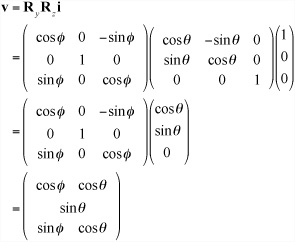
For a one-to-one mapping between values of θ and φ and points on the sphere, θ should take values between 0 and 2π, and φ should take values between 0 and π. Think of them as longitude and latitude. Of course, several other variations on this theme will serve just as well.

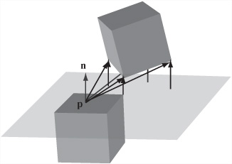
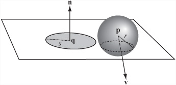
When seeking to detect a moving sphere’s position with relation to a wall or plane surface, as illustrated by Figure 19.1, you formulate the problem mathematically as the intersection of a sphere S(c, r), moving along a vector v, with an infinite plane defined by the point p and the normal vector n. Given this start, you now identify the plane as plane P(p, n).

Figure 19.1. A moving sphere and a plane.

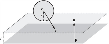
As is evident if you review the discussion in Chapter 8, the technique used to describe the collision of a sphere and a plane is almost identical to the technique used to describe the collision of a circle with a line. First of all, you find the value n · (c – p). If this value is positive, the sphere lies on the positive normal side of the plane. If the value is not positive, it lies on the negative normal side, and in this case you replace n with –n. To make the problem simpler, drawing from a problem solved in Chapter 17, you can find the intersection of a point with a plane. To accomplish this, you offset the plane by the vector rn and find the intersection of the line c + tv with the new plane P(p + rn, n).

Often you’re only looking for a one-way collision with a plane. In particular, when calculating collisions between solid objects, you assume that the normal to each face is pointing outward. This is used in visibility determination. When the normals are pointing outward, you can simplify the problem involving the sphere and the plane because you no longer need to calculate which side of the plane the sphere is on. The sphere will collide with the plane only if the dot product v · n is negative.

Consider situations in which a sphere collided with a moving point or another sphere. Again drawing from the discussion in Chapter 8, to start with, picture the sphere as stationary at the origin, with a particle or object at p moving along the vector v. You now need to solve the equation p + tv = r, which is equivalent to

With this you have a quadratic equation in t. You can solve it using the quadratic formula, and after doing so, you arrive at two possible collision points. To identify the point of collision, you focus on the smallest positive value. If it turns out that one value is negative, then your particle or object is inside the sphere to start with.

Having solved this problem, it’s simple to extend it to two general spheres colliding. As with the case of two circles, the problem of two spheres of radius r and s colliding is equivalent to a particle colliding with a single sphere of radius r + s.

As you move from 2-D to 3-D, given the extra dimension, you find that objects no longer collide along a line. Instead, they meet along a collision plane. The collision normal is the most useful means of detecting the collision. When resolving the collision, only the component of motion normal to the collision is affected. The tangential component is unchanged.

As with finding the collision normal with a circle, finding the collision normal with a sphere is straightforward. The normal lies along the line from the point of contact to the center. When two spheres collide, this line is directly along the vector between the two centers. When the sphere collides with a plane, then the plane’s normal is the collision normal.

An ellipsoid is the 3-D equivalent of the ellipse you explored in discussions of 2-D collisions. As with the relation between a circle and an ellipse in 2-D, in 3-D, one easy way to think of an ellipsoid is as a sphere that has been transformed by a general scale in three dimensions. In this respect, a point on an ellipsoid centered on the origin has the general form v = RSi. In fact, if you include position, orientation, and scale, you can exactly describe a general ellipsoid using a general transform T, applied to the unit sphere described by (cosφ cosθ, sinθ, sinφ cosθ)^T.

In anticipation of the discussion that follows, the term transform is used somewhat loosely in this chapter. At times it is used to describe just the rotation and scale parts of the transform proper, in the form of a 3 × 3 matrix. To keep the position part of the transform separate, for clarity you employ the notation E(p,T). In practice, however, it’s more efficient to use the full 4 × 4 transform. Additionally, as with the 2-D ellipse, you can also describe the ellipsoid by means of a list of its principal axes and the values a, b, c. The two descriptions are equivalent.

Calculating a collision between an ellipsoid E(p,T) moving along a vector v and a point or plane is best accomplished by transforming space so that the ellipsoid becomes a sphere. Given the description of the ellipsoid in the previous section, to accomplish this, you must invert the transform T. After you invert the transform, you then look for the collision between the transformed plane and the unit sphere starting on T^–1p, with a displacement of T^–1v.

This understanding puts you in a position to again approach a problem left dangling at the end of Chapter 8. This problem involved calculating the normal at the ellipsoid (or ellipse) surface. To proceed, recall the discussion from the previous chapter concerning normals. In the case of the plane, the transformed normal T^–1n is not normal to the transformed plane. Instead, it is necessary to use the inverse transpose matrix, which is the transpose of T. Similarly, after arriving at the transpose, to determine the collision normal in world space, you must apply the inverse transpose (T^–1)^T to any collision normals. The ellipsoidPlaneCollision() function encapsulates these operations:

Here’s an example of this method in code:

function ellipsoidPlaneCollision(ell, pl)
   set inverseTransform to inverseMatrix(ell.matrix)
   set inverseTranspose to transpose(ell.matrix)
   set planePoint to matrixMultiply(inverseTransform, pl.refPoint-ell.pos)
   set circleVel to matrixMultiply(inverseTransform,
                          ell.displacement-pl.displacement)
   set normal to matrixMultiply(inverseTranspose, plane.normal)
   set t to circlePlaneCollision(circlePos, 1,
                                    circleVel, planePoint, normal)
   return t
end function

As has been anticipated by the discussion in Chapter 8, the next step in the 3-D version of collisions involves collision between two ellipsoids. Put formally, the question is one of how to find the intersection of two ellipsoids. Based on the difficulties involved with detecting collision in 2-D between two ellipses, it becomes evident that you cannot solve this problem algebraically. However, algebra offers an excellent start. Consider how you can describe this problem in terms of matrix algebra. Suppose your ellipsoids are E₁(0,T₁) and E₂(p,T₂) and the relative velocity is v. You’re looking for two unit vectors u₁ and u₂, which satisfy T₁u₁ = T₂u₂ + p + tv. Taking T₁ to the other side of the equation, you have .

Given this formulation of the problem, you face five unknowns. These are the unit vectors u₁ and u₂, with two degrees of freedom each, and the scalar t. However, to narrow down the solution, you can add one more condition. This condition is that the two ellipsoids must meet at a point. When the ellipsoids meet at a point, at the point of contact the normals must be parallel. Since the normal of an ellipsoid at the point Tu is the point (T^–1)^Tu, you arrive at

Inverting the first transform, this expression becomes

which you can write as u₁ = Mu₂. With this version, you can now eliminate u₁ from the first equation, which tells you that

Since u₂ is known to be a unit vector, between them, these two results form a system of three independent equations in three unknowns. Containing a mixture of trigonometric and linear terms, the equations cannot be solved algebraically. Instead, a numerical approximation method must be used. However, it is still possible to simplify things if the ellipsoids are the same size (have the same transform T) or a scalar multiple of one another (transforms T and aT). If either of these applies, you can invert the transform matrix to turn the problem into a collision of two spheres. This is a problem that you have already solved:

The second equation indicates that the normals are parallel, and from it you know the two results, either u₁ = u₂ or u₁ = –u₂. With the first of the results, one ellipsoid is inside the other. With the second of these results, you can proceed more directly to the solution. By substitution in the first equation, you find that

This follows since u₁ is a unit vector. The remainder of the method follows for the collision of two spheres.

A cuboid has eight vertices joined together by 12 edges, making six faces in all. Think of a brick. As with ellipsoids, you can consider a general cuboid to be a transform T applied to a standard unit cube centered on the origin. Its eight vertices are the eight different combinations of (±0.5 ±0.5 ±0.5)^T. Knowing this transform, it is simple to test whether a particular point p is inside the cuboid. To do so, you find T^–1p and determine whether each of its coordinates has absolute value less than 0.5.

Knowing whether coordinates have absolute values less than 0.5 gives you one method for finding the point of intersection of a line p + tv with the box whose transform is T. You’re searching for the smallest value of t such that T^–1 (p + tv) = T^–1p + tT^–1v + tw lies within the cube. This amounts to six inequalities:

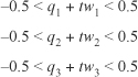
An efficient algorithm exists for solving systems of linear inequalities such as this one. It is called the simplex algorithm. However, this algorithm is very specific to cuboids and is beyond the scope of the current discussion. A more general method is to check for intersection with each of the faces of the cuboid. As with the rectangle, as mentioned previously in this chapter, if you use the dot product of the face normal with the collision vector, you can immediately discount all faces on the other side of the cube from the particle.

How to calculate the point of intersection of a particle with a plane has already been discussed. One outcome of the discussion was that you were provided with a way to quickly calculate the three possible collision points with the infinite planes through each face. You can then check just these points to find which of them, if any, lies within the rectangle of the face. The check involves a method that will work for any planar convex polygon. As illustrated in Figure 19.2, you test whether the point lies on the correct side of each of the edges of the rectangle.

Figure 19.2. Testing whether a point lies inside a polygon.

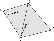
As Figure 19.2 shows, if you find the dot products , you can test if the point P lies on the correct side of AB. If these have the same sign (if their product is positive), then P and C must lie on the same side of AB. If you perform this test for each of the sides of ABCD, you will show that P is inside the rectangle.

The same basic method works for any polyhedron. However, if the faces of the polyhedron are not convex, you must use a more general technique for testing whether P lies on the face. One such method is the raycasting technique discussed in Chapter 10.

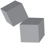
With two colliding boxes, there’s not really much of an alternative to face-by-face checking or, more specifically, face-by-vertex checking. When dealing with boxes at any possible size and angle, several possible face-to-vertex collisions might be used, but with each of them, one of the vertices of one box is in contact with one of the faces of the other. This presents a problem since you don’t need to check all possible vertices, only those at the leading edge of the cuboid. In fact, unless the cuboids are aligned, for each face there is only one vertex that can collide with it. As shown in Figure 19.3, this is the vertex nearest to the face in the direction of the face normal.

Figure 19.3. The colliding vertex.

You can calculate the colliding vertex for each face by calculating the distance of each vertex v of one cube to each face (p, n) of the other. This is the minimum value of (v – p · n). If any of the distances is negative, then there is no possible collision on this face. The same goes for any convex polyhedron. If two vertices are the same distance from the face, then either of them could collide.

Although you might eliminate much work by calculating distances, it remains that quite a few possible collisions will remain to be checked. You’ve also missed out another possible collision, as illustrated in Figure 19.4. This collision occurs when two boxes collide at the edges. This also includes the cases in which an edge of one box collides with the face of another. In this case, there is no vertex-to-face collision at all. A completely different calculation arises.

Figure 19.4. Edge-to-edge box collision.

Approaching the different calculation, as illustrated by Figure 19.5, you can consider the parallelogram swept out by the first edge as it travels along the vector v. If this parallelogram intersects the second edge, then, as Figure 19.5 shows, a collision at point c occurs.

Figure 19.5. Calculating the collision of two lines.

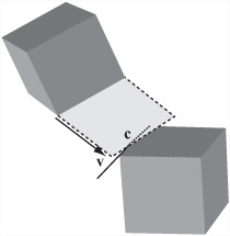
As it is, then, Figure 19.5 depicts a line-polygon collision of the kind already discussed. A collision like this is only possible if the normals of all four of the faces involved have the correct dot product with the velocity vector. The vector is positive for the moving box and negative for the box that is not moving. And as with the vertex-face collisions, you’re only interested in the closest edges.

A sphere can collide with a box in different ways. The sphere might collide with a face, an edge, or a vertex. Collisions with a vertex are straightforward point-sphere calculations. These have already been covered, and with luck, you found the problem simple. Collisions with a face are also simple, and to deal with them, you can adapt the technique already discussed. Toward this end, you first calculate whether the sphere is colliding with the infinite plane containing the face. As with calculations involving polyhedrons, you then check if the collision point is inside the face.

Detecting collisions with an edge is slightly more problematic than detecting those involving vertices and faces. In essence, detecting collisions with an edge involves calculating a collision between a sphere and a line. To set up this calculation, as shown in Figure 19.6, consider a sphere S(p, r) moving along the vector v, and a line (q, u). How do you determine where they meet?

Figure 19.6. A sphere and a line.

One way to simplify the problem given in Figure 19.6 is to realize that you’re interested only in the component of motion perpendicular to the line’s vector. If you subtract the component (v · u)u from the velocity vector and add the vector ((p – q) · u)u to q, you end up with a projection of the problem into 2-D space. Now you’re looking for the intersection of a circle of radius r centered on p with the point q + ((p – q) · u)u. You can then solve this problem using the approaches shown in Chapter 8 or Chapter 9.

As you proceed with your calculations, a few practical measures bear reviewing. To reduce the number of specific calculations needed, you can eliminate several of the sphere-box collisions on the basis that they are impossible. Consider, for example, that face-sphere collisions are possible only if the face normal is pointing in the opposite direction from the velocity. Edge-sphere and vertex-sphere collisions are possible only if at least one associated face normal is pointing in the opposite direction from the velocity.

Mathematically defined, a cylinder is the set of points at a distance r from some line. The line is the axis of the cylinder. The cylinder can be either infinitely long or have two circular caps whose normals are parallel to the axis. The cylinder’s length is defined as the distance between the two caps. The intersection of an infinite cylinder with any plane perpendicular to the axis is a circle. If the intersection is with any other non-parallel plane, the result is an ellipse. You use the notation C(p, v, r, l) to represent a cylinder of radius r centered on p, with axis vector v and length l.

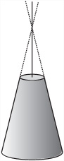
A cylinder is a specific case of a more general shape called a cone. A cone is like a cylinder except that the radius of the two end caps is different. As shown in Figure 19.7, the radius of any circular cross-section is proportional to the distance along the axis.

Figure 19.7. A cone.

Cylinders and cones are examples of what is called a surface of rotation. Such a surface is a 3-D shape that is formed by taking a 2-D profile and spinning it around an axis, like a pot forming on a potter’s wheel. Most 3-D modeling software includes a utility for creating a surface of rotation. In some instances, the utility is referred to as a lathe tool. Chapter 21 provides an extended discussion of surfaces of rotation and related topics.

In previous sections of this chapter, you have already done most of the work required to determine when a sphere collides with a sphere or point. A point colliding with the body of a cylinder is equivalent to a sphere colliding with a line. The previous section dealt with spheres colliding with lines. In general, a sphere with radius r colliding with the body of a cylinder of radius s is equivalent to a sphere of radius r + s colliding with the cylinder’s axis.

The end caps of cylinders introduce the only complication. As shown in Figure 19.8, to deal with this complication, you must find the collision point with a flat circle or disc of radius s and center c.

Figure 19.8. A sphere and a flat disc.

There are various ways to solve the problem depicted in Figure 19.8. All approaches are equivalent. One approach that gives a different perspective on the problem is often useful for collisions with flat (laminar) objects. It is related to the method used for circle-line collisions. Using this approach, consider that at any moment you can calculate the intersection of a sphere with the infinite plane containing a circle or other lamina. The intersection of a sphere with a plane is a circle whose radius depends on the distance of the sphere from the plane.

To present the mathematics, observe that a sphere S(p, r) moving along v intersects a plane P(q, n). You define the distance of the sphere from the plane at time t to be d = (p – q + tv) · n. The value can be positive or negative. If |d| > r, there is no intersection. If there is an intersection, the intersection is a circle with a radius of and a center at p_c = p + tv – dn.

So much for how you can find the collision between a sphere and a disc. Now for the specifics of the collisions. Two possible collisions can occur. With the first, if d = r and p_c – q ≤ s, the sphere collides somewhere inside the disc. From this event, you arrive at the following:

If you find the point of collision of the sphere with the laminar plane, you can use this understanding to check whether it lies within the circle.

With respect to the second type of collision, one involving a sphere and the circumference of a disc, you know that the circle of intersection of the sphere and the laminar plane must be touching. In other terms, expressed mathematically, |p_c – q| = r_c + s. Since you’re looking at a cylinder, you know that the sphere can collide only on one side of the disc. You also know that d is positive. This is not the case, however, with a literally flat disc, such as a DVD.

To find a collision with the circumference, you are looking for t such that

To yield an equation in t, you can replace d by its full dot-product expansion. The only drawback is that the resulting function can’t be solved algebraically. While not solvable algebraically, however, the resulting function does generate output that is nevertheless fairly smooth. Essentially, it is quadratic. With respect to the function itself, it shouldn’t come as a surprise to find no algebraic solution. The cross-sectional circle is similar to a moving ellipse when viewed from the perspective of the disc. Still, the situation can change with changing parameters. If you’re dealing with only a particle of zero radius, you can ignore the possibility of a collision along the circumference.

To calculate the collision of a sphere with a cone, you must take into account the angle of the slope of the sides. As in previous passages of this chapter, while you can expand the cone by r to reduce the case of a colliding sphere to one of a colliding particle, care must be taken when calculating the point of impact.

For simplicity, assume that the cone’s apex is at the origin. The apex is the point at which the radius of the cone is zero. If the cone is not infinitely long, this point might not be part of the physical cone. From the apex, the side of the cone spreads out at an angle α. If the particle is at p + tv and the cone’s normalized axis vector is u, then you can calculate the particle’s distance from the axis to be

The radius of the cone on the plane containing the particle at the time given by t is

When the particle collides, these two values must be equal, giving you an equation for t:

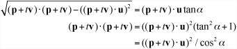
As you can see, this is a fairly minor change to the equation for the cylinder. To transform to the case of the sphere involves similar operations, with the difference that in collisions with the end caps, you can no longer be sure that the distance from the sphere to the cap plane is positive at the moment of collision.

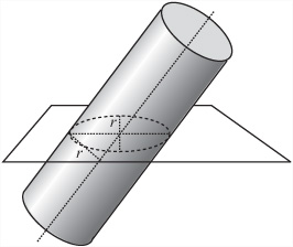
When you’re looking at the collision of two cylinders, a good starting point is to consider the two cylinders as ellipses moving through a plane. You use this approach for collisions along the body of the cylinder rather than at the end caps. To use this approach, first choose a plane in space and project both cylinders onto this plane. It makes things easier if you make a plane that is perpendicular to one axis.

If you set up your problem so that the cylinders are aligned along the same axis, the problem is simple to solve. The problem is then equivalent to two moving circles. If you set up the problem so that the cylinders are not aligned on the same axis, the problem becomes more difficult, for you are then dealing with an elliptical collision. To solve such a problem, you must use numerical methods.

As illustrated by Figure 19.9, to calculate the projected ellipse onto a plane through a cylinder, you first calculate the center of the ellipse. The center of the ellipse is the point at which the plane intersects with the axis. You then have a reading on the halfminor axis. The halfminor axis of the ellipse is always the radius of the cylinder. It is directed along the cross product of the plane normal and the axis. By finding the cross product of this with the plane normal, you can find the vector of the major axis. Using the angle between this vector and the axis, you use trigonometry to find the length.

Figure 19.9. Projecting a cylinder to a plane.

As in 2-D, the most useful technique for calculating collisions of more complex shapes involves creating bounding volumes. A bounding volume is a shape that is known to contain the whole of your object. When the object is already very nearly the right shape, you can use the bounding volume as a proxy for collision calculations. If the object is not close to the right shape, then the bounding shape can at least be used to perform an initial, simpler collision check before performing a full triangle-by-triangle calculation.

The process of calculating a bounding volume in 3-D is similar to the process used in 2-D. To create a bounding sphere, for example, you can average all the vertices of your model to get the center and then calculate the radius as the maximum distance of one point from the center. As with 2-D calculations, this approach won’t usually yield the smallest possible sphere, but it’s quick and cheap. As discussed previously, bounding ellipsoids can be found by a process of factor analysis, and you can create both axis-aligned and object-aligned bounding boxes.

For more collision detection involving complex shapes, generally no better method exists than checking collisions with an arbitrary mesh. The arbitrary mesh consists of a number of vertices joined together in triangles. The normal of each triangle is known and points “out” of the shape. A two-sided mesh has two sets of triangles, one pointing inward, the other outward. Since the direction of the normal is calculated according to the order of the vertices, when you are looking at the triangle, with its normal pointing toward you, the vertices are ordered in a clockwise direction. In many instances, this process can be made less demanding if you create a simplified shape as a proxy, with fewer triangles to calculate.

The technique for calculating collisions with a triangular mesh is essentially the same as for a box. You employ the technique illustrated in Figure 19.2 to determine whether a point is inside a triangle. You assume that if the point is in the plane of the triangle, if it’s on the interior side of each of the three edges, then it is inside of the mesh. This means that the point has to be on the same side as the other vertex of the triangle. Its dot product with the cross product of the edge and the normal must be positive. To express this explicitly, if you set n₁ = n × (v₂ – v₃), then (n₁ · (v₁ – v₂)) · (n₁ · (p – v₂)) ≥ 0.

Translate one or more of the examples in the chapter into a concrete function, and include a function to resolve the collision. Most of the examples are given without code, but with the experience of 2-D collisions, you shouldn’t find this challenge too hard for spheres and boxes.