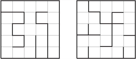
Mathematically, a maze is a kind of graph. However, the term graph is used in a different sense here than you use it elsewhere. As used in this context, a graph is a diagram consisting of a number of points joined by lines, or edges, as shown in Figure 24.1. The vertices formed by the edges are referred to as nodes. Observe in Figure 24.1 that the maze on the left has been converted to a graph on the right. In the graph, each node represents a fork, crossroads, or dead-end in the maze, and each edge represents a path that can be taken from one node to another. There are also two special points, those at the start and the finish. To make things simpler, these are given their own nodes (S and F), although they could just as easily be placed at the nearest branching point or dead end. Although a maze isn’t required to have a start and finish, it usually does.

Figure 24.1. A maze and its associated graph.

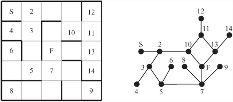
A graph is, in most cases, considered independently of how it’s drawn on the page. When you examine a graph mathematically, you are interested only in its topological properties. In other words, you are concerned about which points are connected to which. However, it is possible to provide a label for each of the edges of a graph. The label can show a number that represents the length of the edge, among other things. You can also label the vertices (nodes) with values that represent some kind of cost or distance. A graph labeled in this way is known as a network. Alternatively, if you do not want to define a formal network, the edge and node labeling can simply be a way to index the graph for reference.

Conventional true graphs can have at most one edge between any pair of vertices, and no vertex may be joined to itself. However, such strictures don’t apply to mazes. In light of this, you need to consider what are sometimes called pseudo-graphs. Mazes sometimes translate to pseudo-graphs. It’s possible to convert any pseudo-graph to a true graph simply by removing offending edges, with no effect on the main properties of the maze, especially with respect to finding a path from one point to another. Since a graph or network is affected by the different choices of edge, it’s important to allow multiple connections when searching for optimal paths. In such cases, you can convert a pseudo-graph to a true graph by inserting additional vertices, which in a network are connected by edges of length zero.

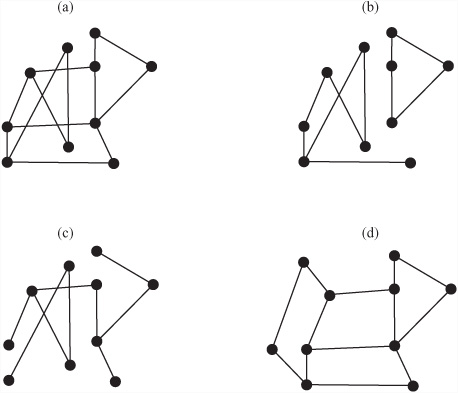
There are a number of other ways to classify graphs that apply naturally to mazes. Figure 24.2 illustrates the different classifications. The following list reviews the classifications illustrated in Figure 24.2:

A maze whose graph is a tree is defined as simply connected. Unless you count backtracking, such a maze has exactly one correct solution. If the graph is connected but not a tree, then the maze is multiply connected. Such a maze contains loops. If the graph is not connected, then there is some set of nodes that can’t be reached from some other set. In other words, the graph can be divided into a number of connected subgraphs that are not connected to one another. For a maze, this means either that it has no solution (if the start and end nodes are in different regions) or that some part of the maze is irrelevant since it can’t be reached.

Graph theory is a large and complex mathematical topic, and it is not possible to explore it in this context beyond what has already been presented. However, you’ll encounter a few graph theory issues in the next two chapters when you look at search strategies.

Although the topology of a maze is the only thing apparently affecting finding a path through it, in reality the physical properties of a maze are also significant. After all, real-life labyrinths and traditional hedge mazes are not generally based on particularly complicated graphs. The classical labyrinth that contained the Minotaur did not have any branching points at all. Instead, it was simply a convoluted path to the center, like the decorative labyrinths used in many ancient mosaics. This understanding is generally considered to underlie the technical distinction between a maze and a labyrinth.

Psychological factors complicate a maze. A game that features a maze that the player looks down on depends for optical complexity on the player’s tendency to immediately seek the goal. If the game is a first-person maze, the difficulty of remembering sequences of twists and turns plays heavily into the success of the player.

Given the extent to which psychological factors are predicated on physical factors, it is useful to provide an inventory of the physical features of a maze. Here is a list of some of the most salient physical features.

Of the salient physical features of a maze, texture is the most subtle. You can explore texture in depth by applying terminology specific to textures. Much of this terminology originated with Walter Pullen, creator of a freeware maze software package called Daedalus. (For more information, see Appendix D.)

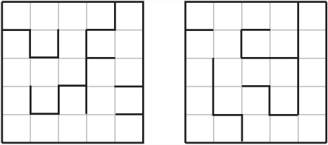
Figure 24.3 shows two mazes with different degrees of what, in relation to texture, Pullen calls river. The maze on the left consists of one long passageway with a few very short dead-end passageways leading off it. Such a maze is described as having a low river. In contrast, the maze on the right is a high-river maze. With this maze, while fewer dead ends occur, the dead ends are longer and more convoluted. Notice, however, that in both mazes the longest path is much the same. You can assign a numerical value to the river by calculating the percentage of dead ends in the maze. In terms of determining how difficult it is to solve a maze, low-river mazes are most difficult. High-river mazes are easier to solve because they offer fewer choices.

Figure 24.3. A low-river maze (left) and high-river maze (right).

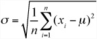
Another term related to texture is convolution. The convolution of a maze can be measured by the standard deviation of the length of a path from any end-node to any other end-node of the underlying tree. Standard deviation is a common statistical tool that measures the average distance from the mean. If the mean of a set of numbers x₁, x₂, ..., x_n is μ, then the standard deviation σ is the square root of the mean squared difference of each number from μ. In other words, the mean is the square root of the variance (which was discussed in Chapter 10). The formula for standard deviation is as follows:

While an extended discussion of statistics lies beyond the scope of this chapter, with relation to the topic at hand, the higher the standard deviation, the lower the value of convolution. The highest convolution is be obtained by a maze that looks like a spider, with a number of paths of equal length radiating out from a central branch point. In this case, the standard deviation of the path length is zero. An alternative measure is the mean distance from one node in the graph to another. A maze with higher convolution tends to be easier to solve although the path to the goal is usually longer.

Figure 24.4 illustrates two mazes. The mazes possess the same degree of river, but different degrees of run. Run is a measure of the twistiness of the maze. Twistiness is an indicator of how far you can travel in a straight line. The run can also be biased in particular directions, resulting in a maze that has a long run in one direction and a short run in another. A maze based on concentric squares, for example, has differently biased run values at different points.

Figure 24.4. Mazes with different degrees of run.

A tile-based maze is based on a grid. Such a maze can be defined as a list of cells with walls between them. For example, a square grid consists of an n × m array of cells, and each cell can have a wall to the north and to the east. To determine if there is a wall to the west of cell (i, j), you look to see if there is an east wall in cell (i – 1, j). A similar technique is used to determine if there is a south wall. You might recall that in Chapter 2 you set up a function for initializing a grid of this kind using the modulo() function.

What applies to a square grid can be applied to other grids. One in particular is the triangular grid. Figure 24.5 illustrates a triangular grid. Grids of this type are best considered as two interlocking sets of cells with different properties or one set of rhombuses (equivalent to squares) that might or might not be split in half.

Figure 24.5. Storing maze data in a triangular grid.

There are quite a few standard algorithms for generating mazes. In general, generating a maze can be done either by growing the walls out from the border or by starting from a (tile-based) maze with all the walls in place and removing walls until the maze is complete. You’ll only consider the first kind here, since it’s more convenient when the maze is set up as suggested in previous sections.

The simplest method for generating a maze is called the recursive backtracker. In this algorithm, you maintain a memory of the path you have taken, and at each stage you look from a neighboring cell to the current cell to see if it has yet been visited. If it has been visited, you try another cell. If it has not been visited, you remove the wall and move into the new cell. If all cells have been visited, you backtrack along your path until you find another cell with an unvisited neighbor. If you get back to the first cell with no more neighbors to reach, then the maze is complete. The recursiveBacktrack() function uses this approach:

function recursiveBacktrack(maze, startcell, endcell, path)
   if path is empty then add startcell to path
   set currentcell to the last cell in path
   set neighborList to the neighbors of currentcell in maze
   randomize neighborList
   repeat for each cell in neighborList
      if cell is not in path then
         set found to 1
         add cell to path
         remove wall between cell and currentCell in maze
         recursiveBacktrack(maze, startcell, endcell, path)
      end if
   end repeat
end function

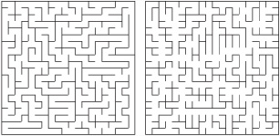
A slight variation on the recursive backtracker method is Prim’s Algorithm, which instead of backtracking, picks a random unvisited neighbor of any cell on the path. This algorithm requires more computational effort, since you must maintain a complete list of all unvisited neighbors. However, it runs somewhat faster and produces a maze with more dead ends. Both the recursive backtracker algorithm and Prim’s Algorithm can be used to provide flood-fill for a paint program. This is so because they completely explore any space designated for them. For this reason, both are convenient methods for creating mazes of irregular shapes or working with any underlying grid. Figure 24.6 shows two mazes created using these two algorithms.

Figure 24.6. Mazes created using recursive backtracking (left) and Prim’s Algorithm (right).

A third algorithm is called Kruskal’s Algorithm. This algorithm works differently from the two already reviewed. Instead of working with a path, it starts by numbering each cell in the maze. Then it picks walls at random. If the cells on each side have different numbers, it removes the wall and renumbers all the walls on each side with the same number. This activity gradually builds connected regions in the maze, until all cells have been numbered the same. At this point, the maze is complete. Prim’s and Kruskal’s Algorithms are examples of what is called a genetic algorithm, which you’ll encounter again in Chapter 26. The kruskal() function encapsulates the actions just described:

function kruskal (maze)
   set wallList to a list of all walls in maze
   randomize wallList
   set idList to an empty array
   repeat for i=1 to the number of cells in maze
      id maze[i] with i
      add [i] to idList
   end repeat
   repeat for wall in wallList
      set cell1 and cell2 to the neighbors of wall
      set id1 to cell1's id
      set id2 to cell2's id
      if id1 <> id2 then
         remove wall from maze
         repeat for each cell in idList[id2]
            add cell to idList[id1]
            id cell with id1
         end repeat
         set idList[id2] to an empty array
      end if
   end repeat
end function

The kruskal() function as presented here can be optimized, but even with optimization, it is harder work for the computer than the recursiveBacktrack() function. Still, it works well and is suitable for a grid of any type or shape.

A fourth function is based on Eller’s Algorithm. Eller’s Algorithm has a few minor disadvantages when compared to those already discussed. Two issues are that it works only for rectangular mazes and tends to have a bias in one direction. Still it’s quick and memory-efficient. With this method, you work through the whole maze a row at a time, using an approach similar to Kruskal’s Algorithm. Each cell in a particular row is given an ID number according to how it is connected to other cells in previous rows. There must be at least one path from the previous to the current row for each remaining ID number, and you can have at most one path with the same ID from the previous row to any connected set in the new row. This is to avoid creating a loop. Generally, implementing Eller’s Algorithm is a more complex task than those discussed previously. Notice that you start with a maze whose walls are all down. The eller() function encapsulates Eller’s Algorithm:

function eller(maze, hfactor)
   set w to the length of a maze row
   set h to the number of rows
   
   // create first row
   set currentRow to ellerRow(maze, w, 1, 1, hfactor)
   
   // create body of maze
   repeat for j=2 to h
      set newRow to ellerRow(maze, w, j, w*(j-1)+1, hfactor)
      set testList to a list of elements from 1 to w
      randomize testList
      repeat for each i in testList
         set id1 to newRow[i]
         set id2 to currentRow[i]
         if id1 <> id2 then
            repeat for each element in newRow
               if element=id1 then set element to id2
            end repeat
            
            repeat for each element in currentRow
               if element=id1 then set element to id2
            end repeat
         otherwise
            add a wall between cell (i, j) and (i, j-1) in maze
         end if
      end repeat
      set currentRow to newRow
   end repeat

   // adjust final row to ensure span
   set idlist to an empty array
   repeat for i=1 to w
      if currentRow[i] is not in idList then
         add currentRow[i] to idList
         remove the wall between cell(i, h) and (i-1, h) in maze
      end if
   end repeat
end function


function ellerRow (maze, w, row, id, hfactor)
   set r to an empty array
   repeat for i=1 to w-1
      add id to r
      if random(1000)<hfactor then
         add 1 to id
         add a wall between cell (i, row) and (i+1, row) in maze
      end if
   end repeat
   add id to r
   return r
end function

Figure 24.7 shows two mazes generated by an implementation of the eller() function using different values assigned to the hfactor variable. A number from 1 to 1000, representing probability, should be assigned to this variable. As Figure 24.7 reveals, this value affects the run factor in each direction and needs to be approximately 50% to create a successful maze.

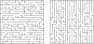
Figure 24.7. Adjusting the random factor for horizontal walls in Eller’s Algorithm (left: 20%, right: 80%).

The greatest advantage of Eller’s Algorithm is that it can be used for a maze of any size in a particular direction. Another advantage is that you don’t need to worry about memory requirements because only one row of the maze at a time needs to be held in memory. It can also be very easily adapted to create a 3-D maze, working one layer at a time instead of one row at a time.

Strange as it may seem, a maze does not become easier to solve by removing dead ends. In fact, it generally becomes significantly harder to solve, not so much computationally as psychologically. Computationally, the faster algorithms work much the same way whether or not the maze has loops, although the simpler algorithms such as wall-following may fail. With a sufficiently large maze, any algorithm based on storing the whole path is going to have memory problems.

Psychologically, the existence of loops means that it is much easier to get lost. If this is a desired property of a maze, however, it invites difficulties, for loops make creating a random multiply-connected maze a difficult proposition. With loops, it is hard to create a random algorithm. Random algorithms, however, generate psychologically interesting mazes. What arises, then, is a tradeoff.

The simplest way to generate a multiply-connected maze is to create a variant of the recursive backtracker algorithm. Using this approach, at the end of each pathway, you open up a wall back into the existing path. While this works well, it also creates mazes with primitive loops. You end up with four cells in a square, for example, or a 3 × 2 group with a single wall in the center.

An alternative method that is much more computationally expensive but more effective begins with a simply-connected maze and then removes walls. To remove the walls, you first choose a few walls at random. For each chosen wall, you calculate the length of the shortest path from one side of the wall to the other. To create a maze with long loops, you can remove the wall with the longest path. For shorter loops, you choose the median path—the one in the middle of the sample. This approach does not lead to a complete multiply-connected maze with no dead ends (a braid maze), but it does produce mazes that are generally interesting. The multiplyConnected() function uses this approach to generating mazes:

   function multiplyConnected(maze, connections)
      // assume maze is already created and simply connected
      repeat with i=1 to connections
         set wallList to an empty array
         repeat for 11 walls in maze
            set s1, s2 to squares on either side of the wall
            set dist to path distance from s1 to s2
            add wall to wallList, sorted by dist
         end repeat
         remove the last wall in wallList
      
      end repeat
      return maze
   end function

For multiply-connected mazes even more than for simply-connected mazes, human-generated patterns tend to be better than anything produced by a random algorithm. Random processes are best used for filling the gaps around the principal areas of the maze with additional convolutions and blind alleys.

Although the grid-based maze is the most common, other maze types can also be used. Topologically, there is no difference between a maze based on a grid and one based on another substructure or no structure at all, but the difference does have implications both psychologically and in terms of computation.

One common maze type that is not grid-based is the circular maze, represented in Figure 24.8. Topologically, this maze is identical to the maze in Figure 24.1, but its substructure is very different.

Figure 24.8. A maze based on concentric circles.

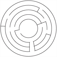
Creating a maze of the form shown in Figure 24.8 can be done in a number of ways, but a particularly effective method entails using a variant on Eller’s Algorithm. With this variant, instead of working row by row, you work circle by circle from the inside out. To work in circles instead of rows is simple. The only change is that regions now wrap from one side of the row to the other. The process is equivalent to creating a maze on a cylinder.

Having created a cylindrical maze, you give it an exit at the top and another at the bottom, and you map the whole thing to a circle. As shown in Figure 24.9, the exit at the bottom leads to the center of the maze, and the exit at the top leads to the outside.

Figure 24.9. Converting a cylindrical maze to a circular one.

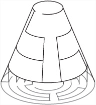
A maze such as the one illustrated by Figure 24.9 won’t be entirely regular in the sense that the walls on the inner circles are more closely packed than the walls on the outer circles. The reason for this is that there are more grid cells in a smaller space. You can offset this problem by varying the horizontal wall density corresponding to the hfactor variable in the previous discussion. Increasing the value assigned to this variable can make more walls as you travel outward.

One further consideration when creating these mazes is how to draw them on the computer. Such drawing is much harder to effectively accomplish than drawing involving a grid of straight lines. In general, making rounded mazes look good requires tweaking by hand. Still, that the automated approach can be effective is demonstrated by the maze in Figure 24.10, which was created using a computer.

Figure 24.10. A circular maze generated by a variant of Eller’s Algorithm.

The main trick to maze navigation requires that you consider each square as a separate room. The situation in many ways resembles working with quadtrees. The only difference is that you have the added advantage that, rather than being arbitrary, the trees constitute an essential part of the landscape. As long as a character is moving within a room, you know that collision is occurring. When the character leaves the room, all you need to do is find which room it is trying to enter and check if a wall is in the way. It couldn’t be simpler.

The details of constructing the code for this section are left as an extended exercise, but one issue that arises is worth mentioning here. This issue concerns a convention of navigation that has become standard in gaming. This convention is referred to as wall-sliding. With wall-sliding, when following a path that naturally takes you into a wall, rather than either stopping dead or rebounding, you remove the normal component of motion but retain the tangential component. The result is that you appear to approach the wall and then slide along it. It’s a very strange concept, but it feels quite natural and is computationally simple.

When working with wall-sliding scenarios in a first-person 3-D view, you must keep the camera a little away from the wall. Otherwise, you’ll get partial views of the room next door. To keep the camera away from the wall, it’s best to treat the observer as a sphere rather than a point.

In a third-person 3-D view, things get a little more complicated because you have different sets of collisions to consider. Imagine a situation in which you have worked out where the character is but still need to determine where the camera will go. Generally, you consider the camera to have a natural resting point, usually somewhere behind and a little above the character. If possible, when the character moves, you want the camera to follow, but often this isn’t possible, as shown in Figure 24.11. As shown in this figure, the character at A has turned, so the camera that was previously at B is now likely to be at C, which is, unfortunately, inside a wall.

Figure 24.11. A camera movement hitting problems with a wall.

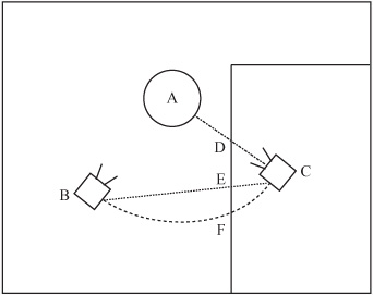
To deal with the situation shown in Figure 24.11, you can treat the camera as another observer following its own path and deal with its collisions exactly as you do with the first observer. But you still have to decide what happens when the collision occurs. The best solution might be for the camera to stop at the point D, the nearest available point along the line AC. This might be a little too close to the observer, however, and you must then lift the camera up into the air so that it looks slightly downward at the observer.

Two alternative positions are the points E and F. With E, the camera first hits the wall on a straight-line path from B to C. On the other hand, F is on a curved path that does not help things. Both of these alternative positions suffer from the same problem. You cannot see everything the character sees.

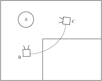
Meanwhile, for a situation like that shown in Figure 24.12, it would be foolish to take any of these options when there is a perfectly good camera position at C. In this case, you might be better off to cut to C in a jump instead of interpolating the camera from B to C and passing through the wall.

Figure 24.12. A perfectly reasonable camera movement running into problems on the way.

As you’ve seen before, these decisions about camera control are very much a matter of preference and require careful handling. If in doubt, make sure your user can override whatever unacceptable thing your particular system chooses to do in some unanticipated situation.

Another reason that grid-based mazes are convenient to work with is that you can calculate relatively easily from any particular point which areas are visible. This, then, is an issue that concerns line of sight. Working with line of sight is useful both for visibility culling in a 3-D FPS and when calculating enemy AI behavior. Picture, for example, a Pac-Man-style ghost or a sentry in a stealth game. To explore this topic, square-based mazes are addressed. The techniques discussed can be used with other mazes, as well.

The simplest way to demonstrate a reason for developing a line-of-sight algorithm is to take a look at a diagram, such as the one illustrated by Figure 24.13. Here, a character is situated at the point marked with a cross. All the places the character can see are shaded. Notice that in addition to the cells along the principal rows, a number of neighboring cells are also partially visible.

Figure 24.13. Visibility determination from a particular point.

It should be immediately clear that even in a grid, the situation depicted by Figure 24.13 requires calculations that are by no means simple. However, there are some useful shortcuts that you can take, particularly in a simply-connected maze. The trick is to make use of recursion. Each time you pass through a doorway, you’re entering a new simply-connected area illuminated by a beam of light defined by the doorway and the beam of light you began with. In other words, you’re splitting the 360° sweep around the observer into smaller and smaller pieces each time a doorway is passed.

Look at Figure 24.13 again. From the point X, there are four possible doorways through which your imaginary light can shine. Two of them are closed, and two are open. With respect to these, the line AB subtends the largest angle at X. (The two points A and B are said to subtend the angle AXB at X.) So you are now looking at the neighbors of the cell marked 2. You see that all three of the doorways are open. At this point, you recurse over each of these. You can go through the door BC into cell 3, splitting the beam further into the angle BXC. Notice that since the vertex D is outside the illuminated angle, you can ignore it. However, since vertex E is illuminated, some light still gets through the doorway DE—specifically, the beam BXE. You also know already that C is illuminated, which means that the whole beam EXC passes through CE.

You continue recursing in this way until you reach either a blank wall or a doorway such as GH. Cell 4 is partially visible, illuminated by the beam FXC, but both G and H lie outside this beam. This means that none of the light from X passes through GH. What’s more, since the maze is simply-connected, you can be sure that none of the light will reach any cell beyond that point.

The visibleSquares() function provides a rough implementation of the line-of-sight algorithm as discussed in this section. One observation is that the function could be much faster, since you’re calculating lots of the values several times over:

function visibleSquares(observerPoint, beamStartAngle,
                           beamEndAngle, fromSquare, thisSquare)
   if beamStartAngle is not defined,
             then set beamStartAngle to -pi;
                       beamEndAngle to pi;
   if thisSquare is not defined then
                  set thisSquare to observerPoint's square
   
   set ret to an empty array
   append thisSquare to ret
   
   repeat for each neighbor of thisSquare except fromSquare
      if there is a doorway from thisSquare to neighbor then
         set v1 to the first vertex of
                      the doorway clockwise from the observer
         set v2 to the other vertex of the doorway
         // find angles of these vertices (in the range -pi, pi)
         set a1 to the angle of v1 with observerPoint
         set a2 to the angle of v2 with observerPoint
         if both a1 and a2 are between beamStartAngle
                                         and beamEndAngle then
         if a1<a2 then
         // vertices are on the same side of the angle range
         set start to max(a1, beamStartAngle)+0.02 --
                           the increment is added to
                           rule out 'just visible' squares
        set finish to min(a2, beamEndAngle)-0.02
        // recurse over all visible squares
        set s to visibleSquares(maze, observerPoint,
                                  start, finish, thisSquare, n)
        append all elements of s to ret
     otherwise
        // the doorway 'straddles' the angle range
        set start to min(a1, beamEndAngle)+0.02
        set finish to max(a2, beamStartAngle)-0.02
        // split the angle range into two parts
        // and recurse along both paths

        set s1 to visibleSquares(maze, observerPoint,
                                   finish, pi, thisSquare, n)
        set s2 to visibleSquares(maze, observerPoint, -pi,
                                   start, thisSquare, n)
        add each element of s1 and s2 to ret
     
      end if
   end repeat
   return ret
end function

Since this version of the visibleSquares() function requires somewhat extended recalculation of values, you might want to think about alternative methods for dealing with the situation in which the doorway straddles the start and end angles. In general, however, there are a number of ways to speed up this algorithm. One is by storing doorway vertex values. Likewise, you might apply Bresenham’s Algorithm as presented in Chapter 22 to avoid the need for floats and trigonometry.

As it happens, the algorithm used in the visibleSquares() function works just as well for multiply-connected mazes; however, you are likely to find that you are sometimes investigating the same square twice from different directions. In fact, it’s more than likely that two parts of the same square might be visible from different sides. The result is that the recursion will often check illumination of particular vertices under several different beams. For a simply-connected maze, the greatest advantage is that as soon as you have determined that a particular cell is out of sight, all passages beyond that cell can be culled from a 3-D scene. This possibility is much less applicable in a multiply-connected maze.

When trying to solve a maze, you face two typical scenarios. The first is when you are placed inside the maze at a particular point and need to find your way to the goal or the exit without knowing anything about the maze. The second is when you are looking down at the maze and trying to find a path from one point to another, often the shortest. You’ll look at the second situation in the next section. In this section, the focus is on the first scenario, which is sometimes called threading a maze. Implementing the algorithm for threading a maze is left to you in Exercise 24.1. The methods that apply to this problem are similar to those you have already encountered when generating mazes.

Exploring the algorithm, threading a maze begins with a classic method for solving a maze that is somewhat strange. It involves turning in the same direction every time you reach a junction. This is analogous to walking along while keeping one hand on the same wall throughout. For any simply-connected maze, this is guaranteed to work. For a multiply-connected maze, it will also work if you are trying to get from an entrance to an exit on the outer walls. However, if there is a loop surrounding the center, it won’t enable you to find a way to the center of a multiply-connected maze. Likewise, it will not find the shortest path. Still, it is computationally simple, requiring no memory of the path traveled.

Another method that is faster than the classic method guarantees a solution in even a multiply-connected maze. This is a simple recursive search. It is the equivalent of the recursive backtracker maze generator. It will follow every path as far as it will go, backtracking and trying alternative paths each time you reach a dead end or a cell you have already visited. It can even be used blind. Blind refers to walking in particular directions and banging into walls. A wall can be viewed as a dead end of length 0.

If you know how to find a path to a goal, then it’s possible to improve on the recursive backtracker approach by preferentially trying to form a path that divides the maze into smaller regions. You might make a path that splits the maze in half. You then know that there is no need to try any path on the wrong side of the maze. This can significantly reduce your search time. This can sometimes also mean that specifically searching for paths that don’t lead to the goal can be more useful in the long term.

Another method that has the advantage of being easy to apply is to use a system of marking. With this approach, imagine walking through an actual maze, making marks on the walls to indicate passages that you have explored. In computational terms, this approach requires that you maintain the whole maze grid in working memory, since you have to be able to annotate the cell data in some way. In all other respects, the algorithm is identical to the recursive backtracker.

To implement the marker method, you make a mark at each junction along the paths by which you enter and leave. A single mark behind you means that you are moving forward. When you turn around, you leave a second mark, meaning that the current path has been completely explored and was unsuccessful. To ensure that each path is explored, you preferentially enter a passage with no marks. As with the recursive method, you also treat all loops as dead ends. When moving forward, if you encounter a junction that you have already visited (as indicated by a marked path), then you turn around. When moving backward, you expect to encounter marks, but there should be only one passageway with a single mark, which is the one by which you leave.

As an added bonus with the marker approach, when you reach the goal, you also have a marked path back to the entrance. You can take the passageways marked once. You can think of this algorithm literally as threading. The marked paths are like a thread that forms loops that indicate dead ends. When you reach the goal, pulling the end draws all the loops of thread in, leaving a single path back to the start.

The flip side of the maze-threading problem is the pathfinding problem. With the pathfinding problem, you deal with two concerns. On the one hand, you know a given maze in advance. On the other hand, you want to find a path, usually the shortest, from A to B.

There are a number of approaches to the pathfinding problem. One approach finds a path at the same average time as the recursive backtracker, but by the opposite method. Instead of searching an individual path to the full before abandoning it (a depth-first search in the terminology of Chapter 26), it searches all paths simultaneously (a breadth-first search). The breadth-first method is somewhat equivalent to Prim’s Algorithm, spreading along a frontier to fill the maze. At each step, you travel one step farther in all possible directions, creating a frontier consisting of all squares at the same distance from the start point. Each cell remembers the neighbor that spread to it, which means that when you find the solution, you can follow the path back to the start. The start is by definition the shortest possible path.

As effective as the breadth-first method is, there is another. This method combines the best of both depth-first and breadth-first searches. It is referred to as the A^* (“A-star”) method. It is implemented in the aStar() function, and it is easiest to explain how its algorithm works if you first examine the code. In code for the function, maze could be anything, as long as you have some way of describing a distance between two nodes. Here is the code for the function:

function aStar(maze, start, goal)
   set pathList to an empty array
   set d to distance from start to goal in maze
   append [d, 0, start] to pathList
   sort pathList on element 1 of paths
   // by estimated distance to goal
   repeat until break
      set path to pathList[1]
      // extend each path to all possible neighbors
      delete pathList[1]
      set currentSquare to the last square of path
      set previousSquare to the second-to-last square of path if any

      repeat for each neighbor of currentSquare except previousSquare
         set p to a copy of path
         // no loops
         if neighbor is not an element of p then
            append neighbor to p
            add 1 to p[2] // length of path
            set p[1] to p[2]+distance(neighbor, goal)
                       // distance underestimate
            append p to pathList // retaining the sort on element 1
         end if
      end repeat
      if pathList is empty then return "No path to goal"
      if pathList[1] ends with goal then return pathList[1]
   end repeat
end function

One of the primary features of the A* Algorithm is that it sorts the found paths according to an underestimate of the distance from the goal. In other words, it sorts according to the length of the path added to the linear distance from the last square to the goal. This technique gives precedence to searches approaching the goal. It is somewhat similar to the “collision halo” approach to collision detection discussed in Chapter 10.

As a further point, it should be fairly clear that although the A* Algorithm is the optimal maze-search algorithm known to date, it still does not give the solution very quickly in a well-designed maze in which paths are specifically designed to lead away from the goal. However, when applied to a random maze, it is by far the fastest algorithm, and it is particularly good at finding optimal local paths—paths to a nearby target. Such a path might be to an AI enemy that is trying to follow a moving target.

To examine the A* Algorithm more in detail, you start with the goal square. At each stage, you take the current best path and extend it to all possible neighbors. If you’ve made a loop, you ignore that path. Otherwise, you calculate the underestimate for the new path and add it back to the list of paths, sorting on the underestimate.

What does this sorting on the underestimate entail? Consider the maze shown in Figure 24.14. In this maze, the path marked by a dotted line is found first by A*, since as it begins it is well aligned. However, along the way, it encounters a few twists and turns, and so its length increases while the distance from the goal also increases. At the moment pictured, the algorithm’s underestimate has for the last time increased above that of the initially less promising path marked with a jagged line. The result is that the algorithm’s attention now switches entirely to the new path, which eventually achieves the goal faster, even though there is a perfectly reasonable route to the goal along the original path.

Figure 24.14. The A* Algorithm in action.

One final observation is that with the A* Algorithm, it’s perfectly possible for a path to get to the goal but be placed somewhere else in the list because another path of maximal underestimate has come into sight.

Create a program that navigates through a maze by either wall-following or recursive backtracking. Draw from the algorithms presented in this chapter.