
Thus far, most of the discussion in this book has involved 2-D problems. While adding a third dimension is mostly just a matter of adding another number, doing so has many implications. For one thing, since your computer screen has two dimensions, not three, when you enter the third dimension, you must find some way to flatten the extra dimension back to a 2-D image. Further, objects in 3-D have sides that are visible and that occlude other sides. To understand how to work with such problems, in this chapter you’ll start by looking at how 3-D space can be represented.
By now you are used to representing a point in 2-D space in terms of a pair of Cartesian coordinates measured along two dimensions (x and y) from a fixed origin. Adding the third dimension (z, for example) involves little more than adding a third number to a list.
As with 2-D geometry, with 3-D geometry you start by creating a space. Creating a 3-D space involves defining three orthogonal (mutually perpendicular) axes and an origin. How you orient the axes is arbitrary. You can point your axes in any direction you like. It is conventional, however, to consider the x-axis as “left to right,” the y-axis as “down to up” and the z-axis as “front to back.” If you move down two units, right one unit and forward three units, your actions correspond to the vector (1 – 23)T.
Note
One of the most common orientations of a 3-D space involves a left-hand axis. With the left-handed axes, imagine grasping the z-axis with your left hand, with the thumb pointing in the positive z direction. Your fingers curl around from the positive x to the positive y direction.
The three-dimensional vector is represented in the same way as the two-dimensional vector. You just add one more component. Most other aspects of vector geometry stay the same. In fact, there is only one addition, which will be discussed shortly. As an example of how 3-D vectors work, consider applying the Pythagorean Theorem. You represent the magnitude of a 3-D vector (x y z)T as ![]() . The dot product is given by multiplying three instead of two components pairwise:
. The dot product is given by multiplying three instead of two components pairwise:

Just as in 2-D space, in 3-D space you can define a line by using a point with position vector p and a direction vector v so that every point on the line has position p + tv for some t. You can also define a plane in 3-D space in much the same way. As shown in figure 17.1, you might employ a point p and two non-collinear vectors v and w, so that each point on the plane is p + tv + sw for some s and t. Another approach is to choose a point p and a normal vector n. The vector n is perpendicular to all the vectors in the plane. While this second method is more efficient, it is less convenient for some calculations. For this reason, in some contexts in this and subsequent chapters, the first approach will be used.

It’s worth noting that the normal gives you a useful equation relating points on a plane. If the normal is (a b c)T, then the points on the plane all conform to the equation ax + by + cz = d, where d is the perpendicular distance of the plane from the origin. This is the 3-D equivalent to the line equation ay + bx = c. In addition, note that if n is a unit vector and p is on the plane, then d = p . n.
Dot products involving 3-D values work much the same way as 2-D dot products. However, when working in three dimensions, you have a new way to combine two vectors. This is known as the vector product, or more commonly the cross product. The vector or cross product is usually designated with a multiplication sign. For example, you represent the vector or cross product of the vectors x and w as x × w. Unlike the dot product, which returns a scalar value, the cross product returns a vector. In other words given two vectors, the vector product returns a third vector that is perpendicular to the two vectors you have used in the product. The result is essentially the three-dimensional equivalent to the normalVector() function introduced in Chapter 5.
Calculating the vector product is a little more awkward than calculating the dot product. The formula for accomplishing this is as follows:

To remember the equation, one approach is to think of it as a determinant represented by a 3 × 3 matrix:

In this matrix, since i, j, k are the basis vectors (1 0 0)T, (0 1 0) T, and (0 0 1) T, each element of the determinant corresponds to one component of the cross product vector. Given this understanding, you can then develop the crossProduct() function fairly readily:
function crossProduct(v1, v2)
   set x to v1[2]*v2[3]-v2[2]*v1[3]
   set y to v1[3]*v2[1]-v1[1]*v2[3]
   set z to v1[1]*v2[2]-v1[2]*v2[1]
   return vector(x,y,z)
end function
Here is a list of some of the most prominent features or properties of the cross product:
The cross product is not commutative. In fact, v × w = –w × v. Nor is it associative. In general, u × (v × w) ≠ (v × w) × w.
The cross product is distributive over addition: u × (v + w) = u × v + u × w.
The cross product of a vector with itself is the zero vector.
If you take the scalar product with either of the two original vectors, if the two vectors are perpendicular, you get zero.
If v and w are orthogonal unit vectors, the cross product is also a unit vector.
Generally, if the angle between v and w is θ, then |v × w| =|v| |w| sin θ.
The magnitude of the cross product of two vectors is the area of the parallelogram whose sides are defined by the vectors. In other words, the area of the shape ABCD, where
 and
and  , equals |v × w|.
The direction of the cross product always follows the same handedness as the axes. Stated differently, if you rotate the space so that the input vectors are aligned as closely as possible to the x- and y-axes, the output vector is aligned in the positive z-direction. As long as your basis maintains the same handedness, the cross-product is independent of the basis.
The cross product, like the dot product, is a useful way to regularize a situation. Regularization involves removing unnecessary elements. For example, suppose you have a plane for which you know the normal n but want to describe it instead by using two vectors on the plane. You can employ the cross product to do this. First, choose an arbitrary vector w that is not collinear with n. Next, take the cross product w × n. This gives a new vector v that is perpendicular to n (and also to w) and that therefore lies in the plane you are interested in. Finally, take the cross product again to get u = v × n. Taking the cross product gives a second vector perpendicular to n, which is also perpendicular to v.
Note
When you work with 3-D calculations, it becomes difficult to remember the distinction between position and direction vectors. A position vector goes from the origin to a given point. Generally, a direction vector goes from a point established by a position vector to another point established by a position vector.
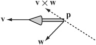
Another common use for the cross product is to find an axis of rotation. You’ll look at this further later, but for now consider Figure 17.2. An arrow at p is pointing along the vector v, and you want it instead to point along the vector w. By finding the cross product v × w, you have a vector perpendicular to both. This serves as an axis of rotation. You can rotate the arrow around this vector to turn it in the right direction. What’s more, by finding the dot product v × w, you can also calculate the angle of rotation.
As a further exploration of the dot products, it’s worth noting one more important calculation. This calculation involves the point of intersection of a line and a plane. Suppose you have a line defined by the point P and a vector u, and a plane defined by a point Q and a normal n. As illustrated by Figure 17.3, your objective is to know a value t, such that p + tu lies on the plane.

There are several ways to discover the value of t. One in particular keeps things simple. Notice that for any point a on the plane, a – q is perpendicular to n. In particular,
(p+ tu – q) · n=0
Because the scalar product is associative, you can reason that (p-q) · n= tu · n. As a result, can also reason that
As you might expect, however, since there is no intersection between the line and plane, this approach fails when u and n are perpendicular. Otherwise, it is quick and reliable.
You can use a similar technique to find the line of intersection of two planes. Accordingly, if two planes are represented by the points p and q and the normals n and m, respectively, then as shown in Figure 17.4, your objective is to find the line that lies on both planes.

To find the line, first notice that since this line lies on both planes, it must be perpendicular to both n and m. Given that it is perpendicular, you can find its direction vector v as n × m. Having gone this far, you now need only to find a single point on the line. To find this point, you apply the previous result. You choose an arbitrary vector in the first plane (a good choice is n × v) and see where the line through p along this vector intersects the second plane. The linePlaneIntersection() and planePlaneIntersection() functions encapsulate these activities. Interactions of lines and planes are attended to by the first function:
function linePlaneIntersection(linePt, lineVect, planePt, planeNormal)
   set d to dotProduct(lineVect,planeNormal)
   if d=0 then return “no intersection”
   set v to linePt-planePt
   return dotProduct(v,planeNormal)/d
end function
The second function attends to intersections of planes:
function planePlanelntersection (pt1, normal1, pt2, normal2)
   set v to crossProduct(normal1,normal2)
   set u to crossProduct(normal1, v)
   set p to linePlaneIntersection(pt1, u, pt2, normal2)
   if p=“no intersection” then return p
   return array(p,v)
end function
Although you need only three coordinates to represent 3-D space, in practice you often use four. There are a number of reasons for this, and discussion of these reasons will be presented in Chapter 18. However, for now, consider that in addition to the x, y, and z coordinates, you add one more, usually designated as w. The result is a four-dimensional vector. This vector follows the rules that have been reviewed for two- and three-dimensional vectors.
While adding a fourth coordinate value might seem arbitrary and confusing, the w-coordinate comes in very handy in a number of instances. The w-coordinate is referred to as a homogeneous coordinate. The term homogeneous means something like “having a similar dimension.” For a position vector, w is set to 1. For a direction vector, w it is 0. To see how this works out, consider the following equation:

The vector from one position vector to another should have a zero w-component. However, at this point, it is not important to emphasize this point too strongly. As becomes clear upon further study, vector addition with homogeneous coordinates is not quite the same as vector addition using only normal coordinates.
Still, to understand the purpose of homogeneous coordinates in 3-D calculations, it’s helpful to briefly draw from a discussion of two-dimensional activities. As shown by Figure 17.5, a two-dimensional plane is defined using axes x’ and y’. The plane is placed in a three-dimensional space with axes x, y, and w, and it coincides with the w =1 plane. As a result, any point (x’, y’) in the plane coincides with a point (x, y,1) in the 3-D space.

However, it’s not just points on the plane that you can map to the 2-D space. You can also compress the whole of the 3-D space onto the plane by a process of projection. As shown by Figure 17.6, for any point P, you draw a line from the 3-D origin through P and find its point of intersection with the plane.

You can even do this with homogeneous points that have w = 0. Although the line OP is parallel to the plane, you still say that it intersects the plane “at infinity.” In other words, it intersects the plane infinitely far along the line on the plane parallel to OP. In all other cases, the point on the plane that corresponds to (x, y, w) is ![]() . In the strictest sense, in fact, there is no difference between the homogeneous points (x, y, w) and
. In the strictest sense, in fact, there is no difference between the homogeneous points (x, y, w) and ![]() .
.
Mathematically, they are considered to be equal. The outcome is that homogeneous coordinates are scale-invariant. If you multiply them by a constant factor, they remain the same.
As an introduction to using homogeneous coordinates, look again at the problem of finding the point of intersection of two lines in 2-D. The line through (a, b) with a vector ![]() can be represented by the equations
can be represented by the equations
a + tp = x
b + tq = y
which give
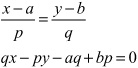
In general, a line in 2-D can be represented as ax + by + c = 0. Using homogeneous coordinates, this is expressed as ax + by + cw = 0. Comparing these two forms of expression, you can see that a line in 2-D corresponds to a plane in homogeneous coordinate space. If you represent two lines in this way, you can find their point of intersection using this approach:
From these operations, you end up with the homogeneous coordinates (br - cq, cp - ar, aq - bp). Notice that if aq - bp = 0, then the two lines are parallel. One resulting observation is that while in standard coordinates there is no solution to the equation, in homogeneous coordinates the two lines meet at a point at infinity with w = 0. Further, the position vector of this point is given by the cross product

The cross product makes sense when you consider that since the two vectors give the normals of the planes in 3-D space, their cross product gives the intersection of the planes. The intersection of the planes corresponds to the intersection of the 2-D lines.
Homogeneous coordinates will be addressed again in the next chapter, where attention is given to how they can be applied in 3-D. Still, it is beneficial to keep them in mind as you read the next section, where I’ll discuss the projection plane for 3-D rendering. The two are closely related.
The process of translating a 3-D scene into a 2-D picture is called rendering. While this is a complex process that you’ll return to at a later stage, at this point, it is worthwhile to consider a few preliminaries, some of which involve the physical media through which rendering is accomplished.
With respect to projection planes, it is helpful first to consider how your eyes receive light reflected from the objects around them. Since light rays travel in a straight line, if you draw a line from your eye out into the world, what you see is the first thing in line with your eye, and your field of vision encompasses anything taken in by the lines coming from you within a particular angle from your eye.
To consider this in light of what happens in the construction of a 3-D world, imagine an observer standing still and looking straight ahead. The world visible to the observer, from the area straight ahead to the peripheral regions on the sides and top and bottom, constitutes the view frustum, as shown in Figure 17.7. The frustum is cut or intersected by different viewing or projection planes. Figure 17.7 shows two planes, the near plane and the far plane.

Note
One of the difficulties in describing 3-D geometry is drawing clear diagrams on a 2-D page. Figure 17.7 shows a 3-D cube transformed into a 2-D picture on the projection plane.
The planes in the frustum are the primary devices used to translate a 3-D into a 2-D image. Referring to Figure 17.7, imagine that an observer is viewing the 3-D world as shown by the projection plane at some distance d. To work out what is to be found at each point of the plane, you can draw a line from the observer and see what it hits. This is called raytracing. For real-time animation, you can calculate where in the space each object is, draw a line to the observer, and see where this line intersects the plane. The precise situation is complicated by lights and texturing, but this is the essential principle.
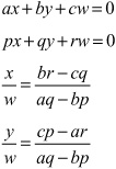
As illustrated by Figure 17.8, to find the point on the projection plane that corresponds to a particular point in space, assume that the observer is facing in the direction n. The point you are interested in is at point p. Likewise, assume that the projection plane is at a perpendicular distance d from the observer, who is at the point o.

Figure 17.8 represents a cross-section, and in it a line is drawn from the point at P to the observer. This line passes through the projection plane at some unknown point. The situation depicted, then, is nearly the same as what is represented by Figure 17.7.
In mathematical terms, the plane normal of Figure 17.8 is the same as the direction the observer is facing. You can find a reference point on the plane drawn at the center of the screen as o + d n, assuming n is normalized. So the point on the projection plane corresponding to P is given by the intersection of the line starting at P in the direction o - p with this plane, which is the point p + t(o – p), where
Note that since n is normalized, n · n = 1.
Having calculated what the projection plane looks like, you can now draw its contents at the correct size on the computer screen, called a viewport. There are a number of different ways you can do this. One way involves specifying the scale. For example, you might determine that one unit of the projection plane corresponds to one pixel on the screen. As shown in Figure 17.9, more commonly you specify the viewport by giving one of the maximum angles in the field of view of the observer, such as the angle θ. In some instances, the whole field of view angle, given by 2θ, is specified.
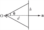
Since you know that tanθ = ![]() , you also know the height of the topmost point on the projection plane. This then becomes a scale for drawing to the screen.
, you also know the height of the topmost point on the projection plane. This then becomes a scale for drawing to the screen.
This approach to calculation, however, can become highly overcomplicated, since you don’t need the value of d. All you actually need to know is the size of the picture on the screen and the angle of the field of view. To make the figures come out correctly, you can then set your projection screen at the appropriate place. Then you simply need to use similar triangles.
You can calculate the distance of the point from the observer along the camera vector to be (p - o) · n and its vertical displacement as (p – o) · u, where u is the “up” vector of the camera. If the projection plane is to have a height of h, then you must also have that ![]() , so the height of the point as projected onto the screen is given by
, so the height of the point as projected onto the screen is given by ![]() .
.
Here’s a function that draws together some of the previous observations, translating a point in space to a point on the screen. As arguments, the pos3DToScreenPos() function takes the observer position and normal, the vertical field of view angle, the height of the screen, and the up-vector of the observer.
function pos3DToScreenPos(pt, observerPos, observerVect,
                             observerUp, fov, h)
   set observerRight to crossProduct(observerUp, observerVect)
   set v to pt-observerPos
   set z to dotProduct(v,observerVect)
   set d to h * tan(fov)
   set x to d*dotProduct(v,observerRight)/z
   set y to d*dotProduct(v,observerUp)/z
   return vector(x,-y)
end function
The pos3DToScreenPos() function returns the point’s position on the screen relative to the center of the 3-D viewport. The position of y is measured downward. Since in practice you precalculate many such values, the function could be made more efficient. In addition, there are also some complications about points behind the observer. On the other hand, in practice you can let your 3-D card handle this part, as will become apparent momentarily.
To explore further how an image is displayed, as mentioned previously, the set of points that is visible to a particular observer is called the view frustum. As illustrated by Figure 17.7 (shown previously), the view frustum is defined in part by the base of a truncated pyramid. A pyramid is a six-sided shape. Its sides are at an angle determined by the field of view. Its front and back faces are determined arbitrarily and are sometimes referred to as the hither and yon of the camera. While you can theoretically see infinitely far and infinitely near, when rendering it is convenient to clip the scene at a certain distance, often using fogging to obscure the distant objects before they disappear from view.
In the equation for screen projection, notice that although changing o and θ both affect the image on screen, they do so in different ways. Moving the observer while leaving θ constant moves the view frustum. It changes the scale of the image linearly. By changing the field of view, however, the shape of the view frustum can be changed. This is like altering the angle of a camera lens. Choosing the correct field of view for your scene can take a little fiddling with the parameters to make something that looks right, just as a director or cinematographer may spend a long time choosing the right lens. None is more correct, but they have different visual effects. The most natural-feeling will be a viewing angle that is the same as the angle the computer user has to the computer screen—but this depends on how near they are to the screen and the resolution they are using.
Perspective is a technique for representing objects on a flat surface. The technique in art of using perspective was mathematically defined during the Renaissance, but the basic principles of perspective had been used prior to that. As defined mathematically, perspective is the approach used to render a 3-D scene on paper. While useful for drawing, however, it must be technically translated if it is to be an effective approach to rendering images on a monitor.
To draw a scene in perspective, you start by creating a horizon. The horizon is supposed to be drawn at the height of the observer’s eyes. Each point on the horizon is a vanishing point. The vanishing point represents an object infinitely far away along a line drawn from the observer’s vertical axis. As shown in Figure 17.10, the classic example of this is a road stretching into the distance.

In Figure 17.10, in addition to the road, a number of lampposts are drawn. If you were to travel along the road, the lampposts would be spaced along the road, as would be the lines on the road. The dotted lines on the left of the figure illustrate the basic technique. Two types of lines are used. Those that begin with the first post and converge at a point in the horizon are called orthogonal lines. Those that represent the lampposts or are transverse lines.
To develop the perspective, you divide the transverse line of the front post into several equal parts, joining each one to the vanishing point using an orthogonal line. You then draw in a line from the bottom of the first post to the top of the post that represents the visible background. Your remaining lampposts are placed so that they coincide with the points where the this line meets the orthogonal lines.
Mathematically, you can calculate that the image size of an object decays exponentially with distance:
Height in image = height × e–k(d–d 0)
where k is some constant and d0 is the distance of an object whose height in the image is equal to its height in reality. There’s nothing special about using e in the equation. Any base will do if you scale k accordingly.
The reason that perspective is not particularly useful in computer 3-D engines is that it requires many recalculations if your observer moves. However, if you’re working with simple scenes and a fixed observer, it can be an easy way to create a quick 3-D effect.
Exploring the difference between drawing and rendering involves seeing how the values k and d0 in perspective drawing relate to d and θ in standard 3-D rendering.
Although the standard perspective projection method described in the previous section is the most common way to draw a 3-D scene, other methods prove more useful in some circumstances, particularly in architectural and technical drawings.
Standard perspective projection is sometimes called central projection. With central projection, something distinctive occurs as you move farther away from the projection plane. As shown in Figure 17.11, as d increases and θ decreases, the objects on the screen always appear the same size, and the view frustum becomes a simple box.

The image shown in Figure 17.11 is called orthographic. When the object you are looking at is at a different angle, it can also be called oblique, axonometric, or isometric, but all these are equivalent to the orthographic view. Only the orientation of the object has changed. In an orthographic view, the distance of an object from the viewer or any other object has no effect on its size. It does, however, affect the position of the object on the screen and the drawing order. Otherwise, all you need to know is the size of the viewport.
In gaming, the most common of these orthographic views is the isometric view. This is where you look down on an object in an orthographic projection at such an angle that each side of the object is at the same angle to the projection plane, so they are all viewed as the same length. (You’ll look at isometric games briefly in Part V.)
One more projection technique is worth noting. Instead of a projection plane, you use a projection sphere or cylinder around the observer. In some ways, you might imagine this to be more realistic. After all, you aren’t actually looking at the world through a window but through two movable eyes. However, using a projection sphere creates some rather strange effects. One example is the Mercator projection of the earth, which is the most commonly seen map of the planet. In a Mercator projection, you imagine placing the earth inside a cylinder of paper and shining a light from the center. The shadow cast on the cylinder forms a map, which you can then unroll.
This is a good way to deal with the problem of mapping a spherical object like the earth onto a planar map, but it has some problems. Among other things, measuring distance is extremely difficult. The farther away you move from the equator, the more spread out the map is, until the North Pole is actually infinitely spread out, and infinitely high up the cylinder. On a map, this is why Greenland is so enormously out of proportion to its actual size. Navigating through a world using this kind of projection would be very weird and confusing.
As became evident in the discussion of 2-D images, it can often be useful to get a list of all objects along a ray. A ray is a line with one point of termination that extends infinitely. Chapter 10 discussed how to calculate the intersection of a ray with a plane. In the next couple of chapters, you’ll calculate ray collisions for both simple shapes and polygonal meshes. In the current passage, it is worthwhile to look at a few applications of this method, assuming that you can employ a 3-D engine to calculate the ray for you.
As anticipated by the discussion in Chapter 10, raycasting is useful in many circumstances, but two are the most common. The first is in user interaction. For example, consider a situation that arises when someone clicks on the 3-D scene and must calculate what object is underneath it. The second is in collision detection. Consider a situation in which one or more rays cast in front of a shape can be used like the beam of a headlamp to determine whether there are any obstacles ahead.
The basic principle of raycasting is that you send a query to your real-time engine, passing it a starting point and a direction vector. The query then returns a list of models with which the ray intersects. Depending on your particular 3-D engine, the query might contain some optimization methods. In some cases, for example, you can specify a maximum number of models to return, a list of models to check against, and a maximum length for the ray. More detailed results might involve collision points and collision normals or the texture coordinates clicked on.
A good example of how this can be useful is in terrain following. Terrain following involves an object that is moving along a ground of varying height. Suppose your ground is a continuous triangular mesh, and you are creating a 4 × 4 vehicle that is driving along the terrain. How can you make the vehicle move realistically across the various bumps? To do so, you must know how high each wheel needs to be, orienting the vehicle accordingly.
One way to assess the heights of bumps is to store the information about the ground as a 2-D height map. This approach provides rapid information, but at the same time, it also requires high amounts of storage space. Another method—which might be quicker, depending on the speed of your 3-D engine and card and the complexity of the geometry of the terrain—is to cast a ray downward from each wheel and orient according to the collision points. This approach has the additional advantage of working equally well with a terrain that is changing over time, such as water waves.
A similar simple example is gunfire. In a first-person shooter (FPS), each player or enemy has a weapon that generally fires in a straight line. At the moment the gun is fired, a quick raycasting collision check determines where it will hit.
The technique is less useful when dealing with objects three or four times bigger than the mesh against which they are colliding. It is also not very useful with objects that are colliding with other objects that may be smaller. In such cases, you must use a large number of rays to determine whether the path is definitely clear. Certain workarounds are available, however. For example, if the objects are significantly different in size, it becomes possible to approximate the collision by using a proxy shape, such as a sphere or bounding box.
Using interaction requires raycasting. The simplest example is when the player of your game clicks on the screen to select an object in 3-D space. How do you determine which object they have clicked on?
By choosing a point on the screen, your user has actually selected an angle for a ray. In fact, you’re running the process of drawing a 3-D point to the screen in reverse. The simplest way to determine this point is to use the projection screen method to find a particular 3-D point under the mouse position. You then use this point to create your direction vector. To do this, as shown in previous calculations in this chapter, you need the field of view angle θ and the height h of the viewport. Then the distance to the projection plane can be found as ![]() .
.
Having found this distance, and knowing the camera’s forward and up-vectors, you can quickly calculate the point under the mouse. The screenPosTo3DPos() function performs this calculation:
function screenPosTo3DPos(viewportPos, observerPos,
                            observerVect, observerUp, fov, h)
   set observerRight to crossProduct(observerUp, observerVect)
   set d to h / tan(fov)
   return observerVect*d - observerUp*viewportPos[2] +
                             observerRight*viewportPos[1]
end function
You now have all you need to cast a ray. The start point is the camera position, and the direction is the vector to the point you found. This tells you the model clicked on.
Suppose you need to drag the model to a new position. This question gives you a technical problem. While there are three dimensions to move it in, there are only two dimensions for the mouse. Somehow, the user’s movements need to be translated into 3-D space.
How the movements are translated depends on the particular circumstances. Consider what happens if the model is part of a plane. It might be an object on the ground, a sliding tile, or a picture on the wall. If this is the case, then your two directions of motion are sufficient. You need only to find a way to constrain the motion in the particular direction.
If the model is free to move in space but not rotate, then the best solution is likely to combine the mouse movement with a key. You might program your game so that the user presses the Shift key while moving the mouse. This might cause the object to move in the camera’s xz-plane rather than the xy-plane. Alternatively, while making the drag occur only in the current xy-plane, you can allow the user to move freely around the object, changing the plane of view or providing multiple views of the same object. Finally, if the model is supposed to be rotating in place, then mouse movements can correspond to rotations in the direction of two axes.
To accomplish such tasks, you can start with constraining to the plane. This is an extension of what you’ve already seen. As the mouse moves, you cast a ray from its current position to the plane you’re interested in. You can use this as the new position for the dragged object, offsetting it by its height or radius as appropriate. As a note, the position does not have to be a on a plane. It can be rough terrain or even other models. Think about the pool game example, which involved a “ghost” ball demonstrating where a collision would occur.
For a more sophisticated variant, you can “fake” the ray position so that the users feel they’re dragging the middle of the object instead of its base. Figure 17.12 illustrates how this might work. First, you calculate the current offset of the base of the object from its midpoint as they appear on the screen coordinates. After that, you apply this offset to the current mouse position to get the ground position you’re interested in. Now you drag the object to sit correctly at that position. The user isn’t precisely dragging the midpoint of the object, but it feels that way.

Dragging the object freely in space is an extension of this. You’ll always have to constrain to a plane. However, you can give a freer choice as to what plane that is. Generally, while the most natural approach involves using a plane normal to the camera, you can also use one normal to the up-vector, or any other vector that seems convenient.
A much more difficult problem comes when you want to allow the user to rotate objects with the mouse. You can start with the simplest of these situations, which is when you want players to be able to rotate themselves, as in a mouse-driven FPS. In that case, a mouse movement corresponds to a camera rotation.
This problem is reasonably easy to solve. This is because there is a straightforward mapping from the mouse movement to the desired movement. At each time-step, you rotate the camera to point along whatever ray is currently underneath the mouse. (You’ll see in the next chapter how to rotate an object to point in a particular direction.) To accomplish this, you must decide whether to keep rotating if the mouse is held still but off-center. You must also decide whether to rotate only when the mouse is moved. In the case of mouse movement, you need to reset the cursor position to the center of the screen each time you move. (With this approach, it is best to hide the cursor.)
When using the mouse to rotate an object in the camera view, things get a little trickier. There is no hard-and-fast translation from one to the other. You can make a start, however. The most natural assumption for someone rotating an object is that the point of the object clicked on will remain under the mouse as it rotates. You can do this as long as you know the intersection point of the ray. The difficulty is knowing which way should be up. As will be discussed in Chapter 18, you can specify an up-vector for a point-at operation. In this case, there’s no obvious winner.
As an example of how to apply such observations, consider a case in which the object to be rotated has position vector p, and the point on its clicked surface has position vector q. Now the mouse is moved so that it defines a ray o + tv from the observer. You want to know which direction to point the object so that it points toward the mouse position. In other words, you want to point the object toward the ray.
To find the correct direction, you need to find the point of intersection of the ray with the sphere centered on p whose radius is the magnitude of q–p. If there is such an intersection, then this tells you the new position toward which the object should point. If there is no intersection, then the mouse is outside the range of the object, in which case you can either continue to rotate or point it as closely as possible toward the mouse. Another way to put it is to say that you point it along a vector perpendicular to the vector v through the plane containing v and p–o.
But what about the up-vector? One option is to use the camera’s up-vector. This works reasonably well, but it leads to problems when you want to rotate the object to align with this vector. Another approach is to use the axis of rotation, but this causes the object to rotate rather erratically. A good compromise is to use the cross-product of the camera’s direction vector and the movement vector of the point.
Create a function that will draw a three-dimensional cube, culling the back faces. While you can determine which faces of a cube are visible by using the normal of the plane, this is a task that is better left for later. For the moment, concentrate on the projection. See if you can work out how to use the cross product to determine if a particular face of the cube is visible. Use the function to make a cube that spins around its center. Look at the effect of using different projection techniques and fields of view.
In this chapter, you’ve had a brief introduction to three-dimensional space and how it works. As you’ve seen, the third dimension can be understood using the concepts used to discuss 2-D objects. What happens, however, is that calculations become more complex due to the extra freedom of movement and because you have to work with an observer who can’t see the whole space.
In the next chapter, you’ll look further into how the space works and extend the matrix math you met in Chapter 5 to deal with the much more complex motions and transformations available to you.
How to extend vectors into three dimensions
The meaning and use of the cross (vector) product
How to find points and lines of intersection between lines and planes
The meaning of the term homogeneous coordinates and how to use them to calculate intersections
How to use different kinds of projection to create your own 3-D engine
How to use raycasting to create user interaction in 3-D space