The most basic type of game in the context of game theory is the zero-sum game. In this type of game, two or more players compete by making a choice of some kind. With the choice, a certain sum of money is given by the losing player(s) to the winning player(s). The aim is to try to maximize winnings (or minimize losses). The term zero-sum means that the total amount of money in the game is constant. Whenever one player gains, another player must lose.

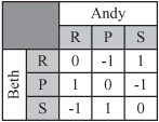
To keep things simple, the games discussed in this chapter will be two-person games. What applies to these simple games applies to games involving more than two players. Figure 25.1 shows a simple example of a two-person zero-sum game. The game is the familiar one of Rock-Paper-Scissors. The game has two players, Andy and Beth. Both players reveal their hands at the same time and have a choice of three options, rock (R), paper (P), or scissors (S). If they match, then no money passes hands. If they do not match, the winner is determined by the system R > S > P > R, where > is used to stand for “beats.” In Figure 25.1, a matrix represents the outcomes. In this figure, the three rows correspond to the three possible actions of Beth. The three columns relate the three possible actions of Andy. The values given in the cells of the table are the payoffs of the payers with relation to the profile of possible actions.

Figure 25.1. A two-person zero-sum game.

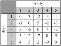
Another example of a game is shown in Figure 25.2. This is a game called Undercut. It is examined by the mathematician Douglas Hofstadter in a book titled Metamagical Themas: Questing for the Essence of Mind and Pattern (Basic Books, 1985). With this game, Andy and Beth have to choose a number from 1 to 5, and the player who chooses the higher number wins the difference of the two numbers unless the numbers differ by one, in which case the other player wins the sum.

Figure 25.2. Undercut.

Not all games are zero-sum. Figure 25.3 shows the matrix corresponding to what is perhaps the most famous game discussed by game theorists. This is the Prisoner’s Dilemma. In the Prisoner’s Dilemma, players don’t compete with each other. Instead, they try to maximize a reward received from a third party. In the usual formulation, they try to minimize the amount of time they have to spend in jail. In Figure 25.3, the payout is listed as a payout vector, with both Andy’s and Beth’s payouts.

Figure 25.3. The Prisoner’s Dilemma.

Theoretically, any zero-sum game can be solved, for each player has an ideal strategy for play that maximizes winnings. Consider, for example, the game of Rube, a matrix for which is shown in Figure 25.4. One difference between Rube and, say, Prisoner’s Dilemma is that Rube clearly makes a fool of anyone who plays it.

Figure 25.4. Rube.

For the game of Rube illustrated by Figure 25.4, imagine that Beth is a carnival cardsharp who offers a maximum payout of $100. Andy is a gullible victim. Andy and Beth choose one of the cards J, Q, or K. The payout matrix is as shown. It should be immediately obvious that Beth’s best strategy is to always choose the King, and Andy’s best strategy is to choose the Jack, meaning that Andy will be paying Beth $1 each time. But why is this the best?

The matrix includes Min and Max values. These represent, for Andy, the maximum amount he would pay to Beth given a particular choice of card, and for Beth, the minimum amount Andy would pay to her (or equivalently, the maximum she would pay to him). In both cases, the values represent the worst-case scenario for a particular card.

Each player’s preferred option is to choose the card that minimizes the maximum payout to the other player. This is known as the minimax strategy. Using this strategy, Andy will choose J and Beth will choose K. Notice that in the payoff matrix, the value of $1 is minimax for both Andy and Beth. This is a stable strategy for each player. If Andy chooses J, then Beth’s best choice of card is K. Any other card will produce a worse outcome for her. Beth is minimaxing the negative value of the table entries.

If Beth chooses K, then Andy can’t do better than to choose J. As becomes evident, then, as long as either player is using this strategy, the other player must also do so. That the strategies of the two players can be paired in this way is called the Nash Equilibrium. One theory derived from the Nash Equilibrium states that every finite, two-person zero-sum game must have either one or infinitely many pairs of strategies with this property. Many games involving more than two players also sustain this dynamic.

With the playing of Rube, the Nash Equilibrium strategy involves choosing a single move every time. The payoff of $1 is called the value of the game, and the game is strictly determined because the minimax for each player is the same. Stated differently, the value $1 in the payoff matrix is both the minimum value in its column and the maximum value in its row. This outcome is called a saddle point of the matrix.

Rock-Paper-Scissors is not determined in the same way. If you look at the payoff matrix for this game, you will see that there is no saddle point. In fact, there is not even a single minimax for either player. The absence of a saddle point means that no single strategy will work for either player. For any choice Andy makes, Beth can make a choice that will beat it. Both players must use a mixed strategy. Specifically, they must choose each option precisely one third of the time and at random. The game is made interesting by the fact that human beings are not very good at picking numbers at random. Given this reality, as you play the game, you can try to notice patterns in the other player’s actions and anticipate them.

When dealing with games with no saddle point, you need a way to determine the appropriate mixed strategy. This requires probability theory. A probability is a number between 0 and 1 representing the likelihood that one event out of a set of events will occur. A fair coin is a coin balanced so that an equal probability exists that it will land either on heads or tails. The probability of throwing heads with a fair coin, then, is 0.5. With a six-sided fair die, the probability of rolling a 6 is 0.167. In general, the probability of a discrete event occurring is given by the following equation:

The chance of throwing a number less than 3 on a single die is , since there are two ways to throw a number less than 3, and six possible events altogether.

Suppose Mary offers that if you pay her $3 per throw, she’ll pay you $1 for each pip that shows on a die. You can calculate the expected amount of money you will receive when throwing the die. This is the average amount you will win per game if you were to play it for long time, and it’s essentially a weighted average:

For Mary’s offer, the expected payout is the sum

Taking off your initial payment of $3, since your expected profit is $0.50, the game is worth playing.

An optimal strategy for a game is a set of probabilities of choosing each of the options such that the expected payout is the same whatever choice the other player makes. For a matrix with a saddle point, the strategy is simple. Choose one option with probability 1. For others, you have to determine the probabilities algebraically. Consider the game of Undercut, played by Beth and Andy, the matrix for which is shown in Figure 25.2. Since the Undercut matrix is symmetrical, you know that the expected payout must be zero. If he picks the number i with a probability p_i, this gives you five equations for Andy’s expected winnings based on a particular strategy:

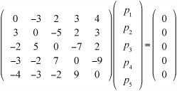
Because the determinant of the matrix for Andy’s expected winning is zero, there are infinitely many solutions to this set of equations, but you also have an additional piece of information. You know that the sum of the probabilities is 1. This sum gives you a strategy for Andy that always has an expected payout of 0, regardless of what Beth does. The same strategy also works for Beth. If you didn’t have a symmetrical matrix and therefore didn’t know the value of the expected payout, you’d solve separately for Beth and include one more unknown, the value of the payout.

The approach applied to the Undercut game can be used to analyze any zero-sum game in which all information about the game is known to both players. For a non-zero-sum game or a game with incomplete information, things get more complicated. If you are interested in pursuing this topic, there is plenty of theoretical work on such problems. An example of a more complex game of this description is Poker.

The information available to players distinguishes different games. A simultaneous game is one in which players choose actions without knowing the actions of other players. Prisoner’s Dilemma provides an example of a simultaneous game. Other games are sequential. In sequential games, each player has some information about the actions of other players. The players take turns choosing an option, until one wins. While fully analyzing sequential games involves complicated work with strings of matrices called Markov Chains, from a computational point of view, a different, less mathematically involved approach can be used.

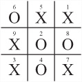
Like Rock-Paper-Scissors, a game that most people know well is Tic-Tac-Toe. In addition to being familiar, Tic-Tac-Toe happens to be an excellent game on which to apply AI theories. Figure 25.5 illustrates a game of Tic-Tac-Toe in which one player, Beth, has won by placing three Os in the second column. Since this is a sequential game, the two players, Andy and Beth, alternate as they play. Each places a symbol in a square of the grid until either the grid is full or one player has three symbols in a row, column, or diagonal.

Figure 25.5. Tic-Tac-Toe.

In Figure 25.5, the squares have been labeled for ease of reference. To explore how game theory applies to the game of Tic-Tac-Toe, consider the minimax concept first. The minimax concept corresponds to the min-max algorithm. To represent the playing of the game, you create a search tree. The search tree works in a fashion similar to the octrees, quadtrees, or the maze networks. Each possible game position in the tree is represented by a node, and nodes are connected by the moves that lead from one to the next. Figure 25.6 illustrates the top of the search tree. Each layer, or level, from the top down represents a move by a particular player.

Figure 25.6. The start of the search tree for Tic-Tac-Toe.

With the representation of a game given in Figure 25.6, notice that some optimizations have been made. Since the game is symmetrical, many of the game positions are equivalent. Andy, the player using x’s, has only three distinct first moves: corner, edge, or center.

To apply the min-max algorithm, you first go through the tree and find all end positions. End positions are those with three symbols in a row. Positions with a win for player 1 are given a score of –1. Wins for player 2 are given a score of –1. Drawn positions get a score of 0. Next, you follow all the links up the tree from these end positions. These links will tell you the possible positions that could lead to your end position. If these occur on Beth’s layer, then you label each node with the minimum value of the nodes beneath. This tells you if Beth can win from this position. If they occur on Andy’s layer, then you label it with the maximum value of the nodes. Figure 25.7 shows a portion of the search tree with these values calculated.

Figure 25.7. Labeling the search tree nodes.

Having completed a pass along the tree, you repeat the process just described, working up the tree until you reach the root node. This will tell you, for each player, the best possible move(s) for any given position. In the case of Tic-Tac-Toe, since both Andy and Beth can force a draw from any of the start positions, all the early nodes have a value of 0.

Given the discussion in the previous section, it becomes possible to lay out a complete set of functionality for solving Tic-Tac-Toe games. The functionality involves a group of five functions that together find a perfect strategy for playing the game. The makeTTTList() and makeTTTtree() functions create the search tree. The other three functions follow up with analysis. Because this is only theoretical and you’re not worrying about speed or memory usage, you’ll save work by not eliminating symmetrical game positions. Here is the makeTTTList() function:

function makeTTTList()
   // creates a list of all possible game boards
   set blist to an empty array
   repeat for i=0 to 5
      set blank to an array of 9 0’s
      if i=0 then add blank to boardlist

         otherwise
         set bl to boardlist(blank, 1, i, 1)
         // list of all boards with i 1’s
         repeat for j=i-1 to i
            if j=0 then next repeat
            repeat for each b in bl
               set bl2 to boardlist(b, 2, j, 1) // i 1’s and j 2’s
               add all of bl2 to bl
            end repeat
         end repeat
      end if
   end repeat
   return blist
end function

Here is the makeTTTtree() function:

function makeTTTtree(blist)
   // creates a tree of all possible moves in blist:
   // for each node, creates a list of all possible parents and children
   
   set tree to an empty array
   set e to array(empty array, empty array)
   add as many copies of e to tree as the elements of blist
   repeat for i=1 to the number of elements of blist
      set b to blist[i]
      // find all parents of b
      if b has no ‘1’s then next repeat
      if b has an odd number of ‘0’s then set s to 1
      otherwise set s to 2
      repeat for j=1 to 9
         if b[j]=s then
            set p to a copy of b, replacing the s with 0
            set k to the position of p in blist
            append i to tree[k][2] // children of i
            append k to tree[i][1] // parents of k
         end if
      end repeat
   end repeat
   return tree
end function

The boardList(), makeMinimaxStrategy(), and minimaxIteration() functions calculate the winning strategy. Here is the boardList() function:

function boardList (board, symbol, n, start)
   // fills a board with n copies of the symbol
   // in all possible ways (recursive)
   if n=0 then return array(board)
   set bl to an empty array
   set c to the number of 0’s between board[start] and board[9]
   repeat for i=1 to c-n+1
      set b to a copy of board
      set k to the position of the next 0
      set b[k] to symbol
      set bls to boardlist(b, symbol, n-1, i+1)
      append all elements of bls to bl
   end repeat
   return bl
end function

Here is the makeMinimaxStrategy() function:

on makeMinimaxStrategy (tree, bl)
   // ‘prunes’ tree by removing all unnecessary children,
   // and returns an initial strategy and minimax tree
   set strategy and minimaxtree to arrays of the same length as bl
   set each element of strategy and minimaxtree to “unknown”
   repeat for i=1 to the number of elements of bl
      set b to bl[i]
      if b is a win for 1 then
         set strategy[i] to “WinX”
         set minimaxtree[i] to 1
         deletechildren(tree,i)
      if b is a win for 2 then
         set strategy[i] to “WinO”
         set minimaxtree[i] to -1
         deletechildren(tree,i)
      if b is full then
         set strategy[i] to “draw”
         set minimaxtree[i] to 0
      end if
   end repeat
   return [strategy, minimaxtree, tree]
end function

Here is the minimaxIteration() function:

on minimaxIteration(strategy, minimaxtree, tree, bl)
   repeat with i=the number of elements of bl down to 1
      // ignore nodes with no parent
      if tree[i][1] is empty and i>1 then next repeat
      // ignore nodes that have already been calculated
      if minimaxtree[i] is not “unknown” then next repeat
      set c to the number of 0’s in bl[i]
      set ply to mod (c,2)
      if ply=0 then set ply to -1
   
      if there is any j in tree[i][2] such that minimaxtree[j]=ply then
         set minimax to ply
         set mv to j
      otherwise
         // find best non-winning move
         set minimax to “unknown”
         repeat for j in tree[i][2]
            set m to minimaxtree[j]
            if minimax=“unknown” then set minimax to m
            if ply=1 then set minimax to max(m, minimax)
            otherwise set minimax to min(m, minimax)
            if minimax=m then set mv to j
         end repeat
      end if
      set strategy[i] to mv
      set minimaxtree[i] to minimax
   end repeat
   return strategy
end function

While the Tic-Tac-Toe system provides a fairly reliable way to compute a winning strategy, it cannot be used all the time, applying it to different games. The reason for this is that it is pretty inefficient. For even a game as simple as Tic-Tac-Toe, there are over six thousand possible positions, and more than a thousand more if you eliminate reflections and rotations. For the games that can be played with boards, the numbers are several times higher. For a game like chess, there are thirty or more possible moves from each position, so the number of possible games is vast—significantly more than there are particles in the universe. To calculate the search tree for chess would take billions of years, and to use it in a game afterward would still take years.

There are a number of ways to optimize the search tree, of which the most important is the alpha-beta search. With the alpha-beta search, when searching through moves at a particular depth, you keep track of two values. One is alpha, the best score you know you can achieve; the other is beta, the worst score that your opponent can force on you.

As an example of how to apply the alpha-beta search to Tic-Tac-Toe, suppose Andy has played squares 3 and 8 and Beth has played square 6. It’s now Beth’s turn, and she has six squares to choose from. Suppose she moves into square 5, the center. It is theoretically possible that Andy will not notice the threat and will play somewhere other than square 4, but it is not likely that this will happen. Instead, Andy’s going to play the correct move and block her. Because you assume that each player will always play the best move they can, it’s no good thinking in terms of the best-case scenario. You must always think about the worst case. Alpha-beta searching means that you focus on the best moves the players can be sure of playing.

If you encounter in the course of a search a node whose value is less than the current alpha value, you know you can ignore it, since you’ve already discovered a better one. Similarly, if you find a node whose value is higher than beta, you can ignore this, too, since you know you’ll never get to play it.

With the current discussion, the assumption of a perfect opponent is somewhat unrealistic when dealing with a human game. In fact, such assumptions are one of the major problems with rational models of game theory and models that involve economics. However, one of the main goals involved in creating an intelligent player is to give the player the tools to play without such brute-force methods. Chief among these is analyzing a board and choosing a move appropriately. In particular, you’re looking for a way to reduce or simplify the search space by performing some kind of pre-analysis to detect promising paths through the tree.

In 1997, one more item had to be struck off the list of things that computers can’t do when the program Deep Blue beat World Champion Gary Kasparov at chess. This was a climactic moment in the history of computers that fulfilled half a century of work in designing AI programs that could play chess.

Chess is one of the most complicated and intractable games, especially given that, just like Tic-Tac-Toe, complete information about the game is available to both players, and no randomness at all occurs. The number of valid games of chess is more than astronomical. It is nearly inconceivable. Given this situation, it didn’t take long for programmers to realize that creating a search tree for chess was impossible. They focused instead on trying to understand how a human being plays the game and how to formalize this into rules that a chess program can follow.

The key insight was that chess is primarily about territory. When grand masters are given a chessboard position to memorize, they can do so very quickly and can reconstruct the board much more accurately than novices. The reconstructions work only for genuine game positions. When the pieces are scattered randomly on the board, grand masters and amateurs perform much the same. Also, when grand masters make an error, the errors are highly global. The pieces are in positions far from where they should be, but the board is left tactically unchanged. The same squares are threated and the same pieces in danger.

The insights concerning territory led naturally to the idea that, instead of analyzing a position in terms of how likely it is to lead to a win, you can analyze it in terms of its current tactical advantage to one or another player. Analyzing for current tactical advantage takes place through estimation functions. An estimation function is basically an equivalent of the underestimate function in the A* Algorithm. Such functions allow you to assign a number to any particular position. By combining this approach with a search tree, you can limit the depth of your search. The result is that you replace the win/lose/draw value with the result of the estimation function for a particular node. You then continue with the alpha-beta algorithm.

Use of an estimation function and a search tree can be combined with more sophisticated methods. For example, you can perform a quick estimation of all the first layer moves. Most of these can be discarded to create a smaller set to be evaluated to a second layer (or ply). When the moves are culled again, only the most promising paths are explored by more than one or two steps. This is also in keeping with the actions of real players. Experts tend not to analyze many possible moves, and bad moves are not only ignored but aren’t even perceived. Even an amateur player won’t consider the impossible option of a pawn moving backward or a castle moving diagonally.

The unavoidable downside of using an estimation approach to limit the search depth is that some winning paths might never be discovered because they look bad at the start. For example, programs that rely on estimation functions find it difficult to discover a winning plan involving a major sacrifice. The immediate loss is much more perceptible than the long-term gain. Still, if this is a problem with a computer algorithm, it is also a problem with human players.

Calculating the estimation function involves a lot of guesswork, plenty of trial and error, and some mathematical analysis, but in essence it boils down to one thing: you need to find a set of measurable parameters that succinctly describe the current position and that might affect your chances of success. Any number of such parameters apply to a chess program. Consider, for example, the total number of pieces (in pawn value) for each player and the number of pieces under threat. More subtle concepts include, among others, control of the center, exposure of the king, pieces in play, and strength of pawn line.

Describing measurable parameters has another advantage. It can be used just as effectively when dealing with games with a random element, such as Backgammon. Even when you can’t determine the moves you’ll be able to use with each successive round of play, you can still classify the strength of your current position. How spread out are your pieces? How many are exposed to capture? The list goes on.

To translate measured parameters into an expression useful for computation, after you have determined your parameters, you must then create a weighted sum of these numbers, which is to say a value a₁p₁ + a₂p₂ + ... + a_np_n, where the weights a₁a₂, ... have been predetermined.

Coming up with such a parameterization is something you have to do as the designer of the program. Since there is no way that you can theoretically calculate the correct value of the weights, you must calculate them by trial and error. The most effective method to calculate by trial and error is to use an algorithm based on natural selection, which will be examined in detail in Chapter 26. Another method for calculation is to use a training system. Using a training system, the program modifies the weights it uses by analyzing the success or failure of particular moves.

To present a simple example of a training system, consider a chess game in action. Two training systems are in place, one for the player, the other for the player’s opponent. Under a certain system of weights, the training program enumerates the value of the current position. Then, looking ahead by a certain number of moves, it chooses the move that maximizes its expected value. At this point, the opponent program makes a move. After the opponent’s move is concluded, the player’s program starts again. If its estimation function for the current position gives a current value equal to or higher than the program expected to be the case, the move is deemed successful and the weight of the parameter that is most involved in the decision is slightly increased. If the current value is lower than expected, the move is deemed a failure and the weight of the responsible parameter is decreased.

Training and learning algorithms are related to the concept of operant conditioning. Operant conditioning is a form of learning that takes place using reward and punishment. It is often associated with the psychologist B. F. Skinner (1904–1990). With operant conditioning, a behavior is reinforced according to its past success. Programs that involve neural networks make use of notions associated with operant conditioning.

With respect to how a training program might be applied to Tic-Tac-Toe, the first step is to suggest a few plausible candidates for measurable parameters of potential success. Here are a few possibilities:

The list of parameters contains some items that conflict with each other. Consider once again the game of Tic-Tac-Toe in which Beth opposes Andy. If Andy plays the top center and Beth plays the bottom center, Beth blocks one of Andy’s potential rows, thus improving her score by criterion 3. On the other hand, by playing a bottom corner, Beth improves her score by criterion 2. Which of these is the better option? There is by no means an obvious answer. To find out, you can use a training process to find out what criterion should be assigned a higher weight. It’s more than possible that one or more criteria might be assigned a weight of zero, meaning that it has no effect on the eventual outcome. You might also find that there are different sets of weights that produce a different but equally effective style of tactical play.

The goal-based approach to AI is similar to the process of programming. You start with a difficult task (“I want to make a first-person shooter”). You then break the task into subtasks (“I need a character, an environment, and some enemies”). Then, you break these up into smaller subtasks, until eventually the tasks are primitive in the sense that they can be programmed directly.

The toughest part of the process involves how to determine the subgoals. It’s not always obvious what steps to take to get to a particular destination. In a game of chess, the goal is “checkmate my opponent’s king,” but breaking this goal into smaller subgoals is a complex task. To accomplish this, the program requires a knowledge base. A knowledge base is as a representation of the world that the program can use to make deductions and judgments. A chess program, for example, might be equipped with advice (heuristics) such as “avoid getting your king trapped,” “try to castle early,” or “if you are ahead, then exchange like pieces for like.” The knowledge base also has some mechanism for deduction, and in particular for speculation. For example, “If I had a castle on that side, it would protect the queen when she checkmates the king.”

Armed with a knowledge base, the program formulates its strategy and, given a particular situation, forms a representation of the strategy and proceeds from there. Among other things, it assesses its goal (“checkmate the king with my queen on e8”). It notices potential pitfalls to the goal (“the bishop on g7 could move in to block it”). It creates a subgoal (“eliminate the bishop”). It searches for a solution to the subgoal (“capture it with my knight”). These actions continue. As it proceeds, the program homes in on a single move that advances the most immediate subgoal.

The goal-based program has more of a resemblance than the tactical approach to a human being playing chess. For this reason, AI researchers held so much hope for the top-down approach in the early days. In fact, this method has had many successes, especially in expert domains. Still, due to scale of the knowledge base required, the goal-based approach has proven hard to scale up into more lifelike areas, such as natural language.

For the obvious reason that every plan has some potential flaw, strategy has to go hand in hand with tactics. No one can anticipate everything, and constraints on computing time mean that every strategy must necessarily contain some blanks. In fact, one of the primary motives for strategic thinking is that you don’t have to worry about calculating every last move. You simply try to advance your position toward some final, nebulous goal. In a game of chess, you don’t care if the queen is protected by the knight or the bishop. You know only that if the master plan is to succeed, the queen has to be somehow protected. However, narrowing actions in this way leaves the door open for an unexpected move to block any plan.

One useful way to combine strategy and tactics is to think of strategy as a particular set of weights in the estimation function of a tactical program. This is not likely to work well in a game like chess, but it will work in a simpler game, like Backgammon. In Backgammon, there are two primary strategies. The first is sometimes referred to as the usual game. With the usual game, you try to protect your playing pieces from being captured as you build up a strong base to trap opposing pieces. When bad luck strikes, it is sometimes appropriate to switch to a different strategy called a back-game. With a back-game, you try to get as many of your pieces captured as possible. While this worsens your position in some senses, it also gives you a strong chance of capturing your opponent and perhaps preventing him or her from reaching the goal. This reverses the fortunes of the game dramatically. While the back-game is a risky strategy and not one to attempt lightly, it can lead to exciting play.

You can model the use of the usual game and the back-game in terms of an estimation function with variable weights. At each stage, the function yields a best possible score under the current strategy. But if this score drops below a particular threshold, the program starts to try out alternative sets of weights. If any of them yield a higher result for some move or for several moves, then the program might decide to switch to an alternative strategy.

When playing against a strategic program, it becomes advantageous to try to induce its strategy from the moves it plays, just as you do when playing a human opponent. In light of this, another important part of strategic play involves pattern analysis. With pattern analysis, you try to determine an underlying principle for the past few moves of a player.

The web furnishes a number of examples of games that use pattern analysis. For example, you can find versions of Rock-Paper-Scissors that will most inevitably beat you. This is possible because humans are poor random-number generators. Such programs search for patterns in your previous moves and extrapolate to guess what your next move will be.

The simplest system of pattern analysis keeps track of each triple move you have made. In the sequence RPRSSRP, the program finds RPR, PRS, RSS, SSR, SRP. The program then predicts that if you have just played RP, you will probably play R. As you play more and more rounds, the program determines that, for example, having just played RP, you are twice as likely to play P as S. It then guesses that this pattern will continue. In general, the longer you play these games, the less well you will do. More subtle systems track whether you won or lost the previous round. In Exercise 25.1 you are asked to create such a program for yourself.

For a more complex game, pattern analysis relies on the program’s strategy module. An example of this might be the question, “What would I do in that situation?” The advantage of asking such a question is that it gives the program a much more powerful way to estimate the likelihood of different moves from the opponent. Moves can even be classified as “aggressive” or “defensive,” which significantly helps with culling of the search tree.

One final example of goal-changing under pressure is the system of scripts. With a script, you follow a predetermined strategy unless an unexpected event occurs. An example of this is a bot in a stealth game. A bot moves in a standard pattern or a random pattern with certain parameters until it hears a noise or discovers a dead body. Then the script for the bot changes, switching to a different alarm or search strategy. The new script might include such goals as “warn the others” or “find the intruder.”

To repeat an earlier definition, top-down AI involves deriving decisions at a lower level from decisions made at a high level. Goals lead to subgoals. With reference to the tree analysis, the principle subgoal of Tic-Tac-Toe is the fork. The fork is effectively the only way to win a game. Below the fork, there is a subgoal of gaining control of empty pairs of rows. These goals coincide with the parameters you use to create an estimation function. This is an appropriate path since situations that are tactically useful tend also to be strategically useful. However, this is also to some extent a result of the simplicity of the game. In a more complex domain, there are levels of description that are beyond the scope of the estimation function. For example, in a game of chess consider the question, “Can the queen reach square b5?” The usefulness of this question depends on your current goal. For most strategies, it will be a completely irrelevant question, so it would constitute a useless addition to the estimation parameters.

With Tic-Tac-Toe, your primary goal might be “create a fork,” but a subgoal is likely to be “create a fork between the left and top lines.” With such subgoals, you then arrive at a further question: “Is the top row empty?” If you are using an estimation function, such a question is not going to be useful. It is useful, however, if you have created a strategy.

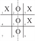
To explore this scenario in greater detail, consider Figure 25.8, which illustrates a complete game of Tic-Tac-Toe with the moves numbered.

Figure 25.8. A strategic game of Tic-Tac-Toe.

One again, the two players are Andy and Beth. At the start of the game, Andy begins with a blank slate. His goal generator immediately starts looking for a possible fork, and he decides to play the corner square 3. Such a decision is based on probability. From his knowledge base, he knows that a good route to a fork using a corner square is to get the corner 7, forcing Beth to move in the center and leaving him open to move in one of the other corners, making a fork on two edge rows. This is his current strategy.

However, consider the difference between tactical thinking and strategic thinking. When thinking strategically, you are mostly thinking in terms of best-case scenarios. You are thinking about what you would like to happen if your opponent doesn’t guess what you’re up to. In the game theory approach, you think in terms of the worst case and assume your opponent will do the worst thing possible from your point of view. Of course, you need to think about your opponent’s reaction when deciding which strategy is best. There’s no point choosing a strategy that is bound to fail.

Beth, too, knows the three-cornered fork trick, so she knows that she can’t let Andy force her into such a situation. Since the easiest way to foil it is to block the diagonal, she considers placing her next move in the center. She realizes that this move would also be a useful step toward creating her own fork, with three pieces in some corners.

Andy’s original strategy is now partially damaged. Since he can no longer force the fork on Beth, he must now find some other way to take advantage of his original move. However, all is not lost because he still has partial control over the top and right rows, and there are only two other rows not controlled by Beth. This leaves him with two possible forks. One move, in corner 7, leaves both of them possible. While this is the move he was aiming toward before, at this point he’s taking it for a different reason.

Incidentally, note that Andy’s move damages Beth’s strategy. One of the rows she wanted to use, on the bottom, is now unavailable. An alternative is available on the left. This makes it so that her only possible rows are the two in the center and the remaining diagonal. Further, there is no way to create a fork without forcing Andy to stop her. Her only option is to force him to a draw, so this becomes her new primary strategy. A quick prediction shows that if she plays a corner, he will fork her, so she has to play one of the edge pieces. From here on, play is predetermined. Each player is forced to play moves that block the other.

Ultimately, such analysis is overkill, but to some extent, it enriches the experience of what it is to play the game, consciously moving back and forth between strategic and tactical perspectives.

Perhaps the purest example of connectionism is the neural network (or just neural net). A neural net is like a simulated massively parallel processing computer. Such a computer is made up of lots of smaller computers modeled on the nerve cells in the brain and called neurons. These artificial or simulated neurons are joined together in a network with input and output and trained to produce appropriate results by a learning process.

To understand how neural nets work, consider the Figure 25.9, which shows a line drawing of a neuron in your brain. A neuron is basically a simple calculation device. Each neuron has a main cell body or soma. Approximately a thousand filaments called dendrites lead into the soma. The dendrites provide input to the soma. For output, the neuron has an axon, which is attached to a side of the soma. The axon in turn splits into various filaments called terminals. As with the dendrites, there are roughly a thousand terminals, and each terminal ends in a small nodule called a terminal button. The terminal buttons are connected to the dendrites of other neurons via an entity called a synapse.

Figure 25.9. A neuron in the brain.

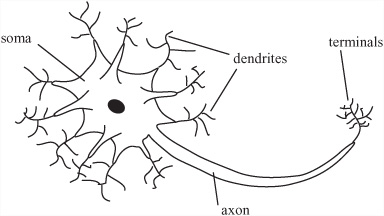
The neuron works by chemical-electrical signals. At any time it can fire or send a signal of a certain strength down the axon. The strength of the signal is always the same for a particular neuron, although the frequency at which the signals are sent can vary. Whether a neuron fires at a particular moment depends on the signals coming into the dendrites.

At any moment, the neuron will fire if the total signal coming into the dendrites is above a certain threshold. The sum is weighted according to the behavior of the dendrite. Some dendrites are excitatory, meaning that a signal received will be added to the total sum. Others are inhibitory, meaning that the signal is subtracted from the total sum. There is also some additional processing that interprets several rapid weak signals as a single stronger one.

After the logic of the neuron was understood, computer scientists sought to use it in computing. To create a neural network, you must model an artificial neuron. An artificial neuron lacks most of the complexity of a biological neuron. The actions of dendrites, terminals and other elements are replaced by a single function as shown in Figure 25.10.

Figure 25.10. An artificial neuron.

The artificial neuron has a certain number of inputs, each of which has an associated weight. It can be given a stimulation threshold that determines whether it will fire. Likewise, it has an output that can be connected to any number of other neurons. At each time-step in the neuron program, you determine the output strength of each neuron by calculating the weighted sum of the inputs and seeing if they exceed the threshold for firing. If the neuron fires, the output can be either discrete, 1 or 0, as in the brain, or it can vary according to the size of the input.

You can avoid some worry by assuming that the total sum of inputs is passed through a limiter function. The limiter function constrains the output to a value between 0 and 1. For a discrete output using a threshold, this is a step function that outputs 1 if the input is greater than a certain value and 0 if it is not greater than a certain value. For variable output, you usually employ one of many versions of the sigmoid function . The neuralNetStep() function provides an example of how to accomplish this:

function neuralNetStep (netArray)
   set nextArray to a copy of netArray
   repeat for each neuron in netArray
      set sum to 0
      repeat for each input of neuron
         set n to the source neuron of input
         add (weight of input)*(strength of n) to sum
      end repeat
      set strength of neuron in nextArray to
                    limiterFunction(sum, threshold of neuron)
   end repeat
end function

Having set up a function for the neural net, you must provide the network some kind of connection to a problem. As illustrated by Figure 25.11, to do this, you create an input layer of neurons, which are connected to the source. The source might be a visual display or the values of a problem. You also connect the input layer to an output layer. The output layer might be a second visual display. Between the input and output layers, you place one or more hidden layers. This creates a multi-layer perceptron (MLP) network.

Figure 25.11. A multi-layer perceptron.

In Figure 25.11, the network might be described has having the problem of calculating the emotional state of a photographed face. It can classify the face as smiling or frowning. The input nodes are given a strength according to the grayscale color of the pixels in a bitmap, and the answer is determined by the output strength of the single output neuron, from 1 (smiling) to 0 (frowning). A more complex network could have more output nodes.

Each neuron in a layer is connected to every neuron in the neighboring layers, so information from one layer is available in some sense to every neuron in the next. In this kind of model, there is no feedback. No neuron can pass information back from one layer to an earlier one. This makes training the network easier, as is discussed in the next section, but it is unrealistic when compared to what happens with neurons in the brain.

Given a particular problem, you need to train the network to solve it. The interesting thing about the neural net approach is that the neural net program knows nothing about the problem it is to solve. There are no explicit procedures or rules. All of the answers emerge from the interaction of all the neurons. As a result, training the network amounts to creating a computer program by an evolutionary process.

The key trick in training an MLP or other simple network is called back-propagation. Rather like the training method you saw earlier for the alpha-beta search, back-propagation works by a kind of behavioral conditioning. You give the network an input and reward it for an output close to the one desired. On the other hand, you punish the network for an output that is incorrect. The rewards and punishments consist of alterations to the weights of the network that improve the results the network delivers.

With the smiling-frowning detector, say that you seek to train it on a particular image. Suppose that after you feed the image to the input layer as a set of color values, the output neuron gives you a value of 0.62. You wanted the output value to be 1, however. The error value is 0.38. You now feed this value backward through the network.

The idea is to adjust the weights of each layer so that they produce a better result with each pulse of the network. You start by altering the weights of the output layer so that as it receives input, it produces a result closer to the expected value of 1. You trickle this effect back to the hidden layer(s), altering their weights to produce a value closer to the desired value. The process is similar to the training process discussed previously. In fact, a neural network is a useful way to create the estimation function for an alpha-beta search.

It’s also possible to train a neural network by using an evolutionary mechanism, “mating” different networks to produce child networks and then selecting the best results from the offspring. This is a variant of the genetic algorithms explored in the next chapter.

At a level more advanced than neural networks is a brand of connectionism that is based on the idea of small interacting subprograms often called actors or agents. This approach is popular among object-oriented programmers. An actor, like an object, is a self-contained entity in the software space that can be treated as autonomous. It has a simple behavior, but because it can interact with other actors in various ways, the overall effect can be to produce complex higher-level behavior.

An example of the use of actors is the bulletin board model. With the bulletin board model, actors interact by posting messages on a bulletin board. Other actors can pick up these messages. The messages are marked with an urgency and contain information or goals that must be achieved. Different actors might or might not be able to use the content of the messages. Another type of bulletin board provides a blackboard with messages written on it for all actors to see. Actors may erase or alter existing messages in light of their own knowledge.

The common feature of all these connectionist approaches is emergence. Emergence allows for higher degrees of organization to bubble up from interactions of simple elements. Emergence is an exciting phenomenon of interest mostly to the strong AI camp. Understanding it is worthwhile when looking at any contexts in which many individuals interact. Such contexts include traffic, crowds, and economics.

One example of emergence involves modeling of flocking behavior. Flocking behavior involves the motion of flocks of birds, schools of fish, or herds of animals. An early and extremely influential model of flocking was given by the Boids program, created by Craig Reynolds. The Boids program featured a number of simple “organisms” that followed just three rules:

A number of other rules can be added, such as avoiding predators or searching for food, but even with these three rules, you see surprisingly realistic flock-like behavior, suggesting that such rules might be behind the motion of real flocks. The boid model has been used for computer graphics and games, and most notably in films such as Jurassic Park (1993). More complex actor-based systems are used for battle simulations such as were seen in the Lord of the Rings film trilogy (2001–2003).

A final method is worth mentioning. Douglas Hosftadter has worked on a process called high-level perception. High-level perception involves building up a representation of a situation under various top-down pressures. This approach is more or less halfway between the bottom-up and top-down approaches. The system uses a number of code objects called codelets that search for patterns in data. The codelets use criteria in a shifting network of associations called the slipnet. The slipnet contains all the concepts the model understands, such as “sameness,” “difference,” “opposite,” “group,” and it uses them to build up a picture of the particular situation. What is interesting about this model is that it can “perceive” a situation differently according to different circumstances. For example, “abc” might be seen in one context as a “successor-group” of letters but in another as a “length-3 group.” This intertwining of perception and cognition is intuitively very lifelike.

Tic-Tac-Toe does not lend itself well to the bottom-up approach. A neural network could of course be used in place of the estimation function for the alpha-beta search. If this were used, however, it would be unlikely to be an improvement, and there is very little analysis of the board position for the actors to share between them. This isn’t to say that a bottom-up approach wouldn’t be interesting, but it wouldn’t be useful as a way to create an intelligent program, as compared to the other approaches.

One method that could be successful would involve creating a neural net that takes any board position and returns the next. This would involve a slightly unusual training regime. Instead of presenting it with a single stimulus and evaluating the response, it would have to play a complete game and be evaluated according to whether it won or lost.

Create a pattern-matching program that plays a game of Heads or Tails against a human opponent. You might use any of the approaches discussed in this chapter, but the easiest is the method mentioned in the section on top-down AI.

Create a simulation of flocking boids. The three rules described in the chapter are fairly easy to implement and produce satisfyingly lifelike behavior, especially in 3-D. You might like to play with adding predator avoidance rules as well.