
You’ve already seen how a 2-D matrix can be used to describe a sequence of transformations in 2-D space. In this chapter, you’ll look at the 3-D equivalent of this, the transform. You’ll also see how transforms can be used to create objects with relationships to each other.
The 3-D world is populated by objects called models. Models are sets of vertices joined together in triangles to make a mesh. In order to work out where these models are, the 3-D engine treats them as a single object called a node. The node is associated with a particular location and orientation. The 3-D engine works out the positions of the vertices relative to the node. The same method is also used to describe the location of lights, cameras, and other members of 3-D space.
To describe a node, you must know three things: its position, its rotation, and its scale. Rotation and scale can be handled by a transformation matrix. Position is a simple vector. The simplest way to visualize this combination of transformations is as a single process acting on the “raw” model. The first action is scaling. The second is rotating about the origin. The final is translating to the correct point.
All of these transformations are affine, meaning that if two lines are parallel before transformation, then they remain parallel afterward. Shears and reflections are also affine transformations. In fact, any transformation that can be performed by a matrix is affine. Rotations, translations, and reflections are slightly stricter. They are rigid-body transformations because, as well as affinity, they preserve angles between lines in space. In other words, while the relative positions of vertices may change, the angles between them remain the same. As illustrated by Figure 18.1, this is not true of scales in general.

Scale is the transformation that is easiest to visualize. Scaling an object by a constant factor involves multiplying each position vector by the scale factor. In terms of matrix mathematics, the matrix is multiplied the matrix nI, where I is the identity matrix. More generally, you can scale by different amounts in each direction. To accomplish this, you multiply the vectors by the following matrix:

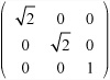
Any scale transformation can be calculated in this way. For example, a scale factor of 2 in the direction (1 1 0) is equivalent to the scale
Rotation is more complicated than scaling. In two dimensions, rotation about the origin is relatively straightforward. It is described by a single angle. When a third dimension is added, however, you must specify an axis of rotation. Any vector in space can act as an axis, but as with the pool balls you looked at in previous chapters, due to topspin and sidespin, any rotation can be decomposed into simpler rotations about the basis vectors.
A rotation about one of the basis vectors can be described by a matrix like this:

Combining all three such matrices gives you a generic rotation:
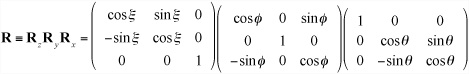
Note
The triple bar symbol (≡) here means “is defined as” or “is identical to.” It’s like a stronger kind of equals sign.
Multiplying out all these matrices is an extremely involved process, but it’s not as bad as it might seem. Suppose you transform the vectors i, j, and k under R. You end up with the column vectors u, v, and w of the matrix. One feature of a rotation is that the vector between a point and its image must always be perpendicular to the axis of rotation. As a result, if you now take the cross product (u – i) × (v – j), you find a new vector a perpendicular to both. This vector a is the overall axis of rotation.
What’s more, you can calculate the angle of rotation α by finding the components of i and v perpendicular to a. In other words, you find the result of projecting vectors i and v to a plane normal to a. Here is how this can be accomplished:
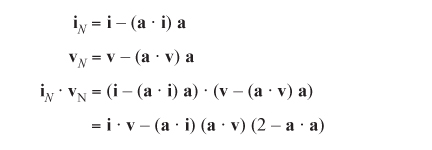
Note
This only works if i (and therefore v) is not parallel to a. If it is parallel to a, you must use a different basis vector for comparison.
Assuming a is a unit vector (if it is not, you can normalize it), and given the definition of rotation, noting that the dot product with i and v must be equal, you arrive at this equation:
Cos α = i · v –(a · i)2
This process can always be used to combine two or more transformations into one. Conversely, since you can decompose a rotation R into primitive rotations about the basis vectors, a rotation is often described by means of a rotation vector giving the angle of rotation about the three axes. You’ll be coming back to this issue several times over the course of this section.
While the notions proposed in this section work fine, you still eventually hit a snag. How can you represent translations? It would be good to be able to perform a complete transformation in one step, including translations. Otherwise, among other things, any combination of transformations would require first translating back to the origin, performing rotations and scales, re-adding the position, and then translating again. Since position information is additive, however, and not multiplicative, such activity becomes seemingly impossible.
The solution to this problem is to use the homogeneous coordinates introduced in the previous chapter. With the aid of the fourth dimension, you can perform translations using a 4 ×4 matrix. Here is how this is done:

Notice that the last row of the calculation is almost irrelevant. It serves largely as a piece of bookkeeping. Also, notice that if you perform a translation on a direction vector instead of a position vector, so that the w-coordinate is zero, the vector is unaffected by the transformation.
If you combine the resultant matrix with the scaling and rotation matrices mentioned previously, you end up with a generic transform
T = PRz Ry RxS
where P is a translation, and S is a scale that appears like this
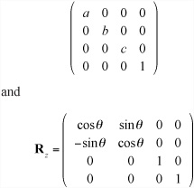
A similar relationship applies for Ry and Rx. The non-translation matrices are created simply by replacing the 3 ×3 matrix at the top-left of the 4 × 4 matrix with the appropriate 3-D matrix.
Because its bottom row is always (0 0 0 1), T has 12 unknown entries. However, not all such matrices are valid transforms. Those with a determinant of zero are invalid. Of the rest, exactly half would perform a reflection and most others would create some form of shear. It’s easy to see that there are nine degrees of freedom in creating a valid transform. Three are rotation angles, three are scale factors, and three are translation values.
Each of the matrices that make up a transform can be inverted fairly easily. For a translation, replace each value with its negation. For a rotation, negate the rotation angle. For a scale, replace the scale factors by their reciprocals. In fact, as it happens, inverting translations and rotations is even easier than that. Their inverse is actually their transpose. In such situations, you say the matrices are orthogonal, which is equivalent to the rigid-body nature of the transformation. This means that you can invert the whole transform. When you do this, it is important to remember that you must apply the inverses in the opposite order:
This process is straightforward providing that you keep track of the primitive transformations making up the transform. Otherwise, you have to either decompose the general transform into its component parts or invert it as it stands.
To decompose a transform into position, rotation, and scale information, you first strip off the translation element from the last column of the matrix. To calculate the scale and rotation, notice first that when you multiply S by the basis vectors, you multiply the basis vectors by the scale factors a, b, and c. For example, RSi = R(ai) = a(Ri). Also, since R is a rigid rotation, Ri is a unit vector.
A further point is that Ri is also the first column of R. Given this information, a must be the magnitude of the first column of RS, and the first column of R is the normalized version of this vector. Since the case is similar for b and c, you can split the transform into the three underlying transformations.
Further decomposing R into rotations about the three axes is also possible, although not always necessary. You’re looking for θ, φ, and ξ such that

(Since it is not involved in this transformation, you ignore the w-coordinate.)
Since the z rotation doesn’t affect the z-coordinate and the x rotation doesn’t affect the x-coordinate, you can see that z1= –sinφ. This tells you the value of φ. Having done that, you can see that z2 = –cosφ sinθ, which gives you θ and x1 = cosφ cosξ, which gives you ξ. The only problem is that there is more than one set of solutions to this system, so different sets of rotations will combine to give the right answer. This might seem trivial, but it does cause problems, particularly when interpolating transforms.
One advantage to working with the raw transformations underlying a transform is that they provide you with a validation system against rounding errors. Because of the redundancy in the transform matrix, small errors can accumulate to give a transform that is not valid if a small sheer factor is introduced. You can counteract this by checking a transform against its underlying transformations and ensuring that the two are true to one another. To some extent, this decreases the value of combining transforms into a single matrix. In this respect, it is important to remember that the main value occurs when applying a transform to multiple objects in a scene. In such cases, a validation isn’t necessary. You need only to validate the transform when modifying it in some way.
Transforms simplify 3-D calculations enormously. This section provides a few examples of how this can be accomplished.
In practice, it’s easiest to work with transforms by ignoring the full transform matrix and concentrating on the underlying raw transformations. In general, you’ll have some node with a transform T, and you’ll want to move it somewhere else. The only time you need to use the full transform is when calculating the actual position of the vertices of a model. For example, the basic unit cube has eight vertices at the eight permutations of the homogeneous vector (±0.5 ±0.5 ±0.5 1)T. You can use a transform to move this cube to any other position or size in space. Once you have calculated the appropriate transform, you multiply it by each of the vertices to determine the new location of the cube.
The same process also works for direction vectors. As a result, the vector along one side of the cube will be unaffected. However, you do need to be careful about normal vectors. Because the scale transform does not preserve angles between lines, a direction vector that is normal to a line or plane before transforming is unlikely to still be normal afterward if the transform includes a scaling element.
If you know that n and v are perpendicular vectors, to find a vector normal to the transformed vector Tv, you must find some new transform Tn,such that TnnTv = 0. Recall from the definition of the dot product that since n · v = uTv, (Tnn)T (Tv) = 0. Likewise, nTTnTTv = 0 Since n and v are perpendicular by definition, if TnTT = I, then the equation is solved. You can conclude, then, that T n = (T–1)T, the inverse transpose of T.
Yet again, it should be stressed that since such calculations are mostly handled behind the scenes by a decent real-time 3-D program, you don’t need to worry about them. Still, it is worth keeping them in mind. They become more relevant as you work more deeply into the details of collision detection.
To consider examples of how you can use transforms to perform a common task, consider the action of aligning an arrow to point at a particular position vector. Suppose the arrow is a model whose root position (its appearance under the identity transform) is as shown in Figure 18.2. Notice that it is pointing along the positive z-axis.
Imagine that the arrow in Figure 18.2 is located at position p, pointing along the vector v. To calculate v, you start with the transform of the arrow. If you know the transform of the arrow, then v is the normalized third column of the transform matrix. You want the arrow to point at a point q instead along the vector v, so you rotate it appropriately. To do this, you can first calculate the vector q - p. This is the new direction for the transform’s z-axis. Normalized, you call this u. Taking the cross product u×v, you can find the axis around which you would like the arrow to rotate. By taking the dot product u · v, you can find the cosine of the rotation angle.
Now all you need to do is to perform the rotation. The general matrix for rotating around an arbitrary axis is a little ugly. It appears as follows:

where the axis is given by the vector (a1 a2 a3)T. If the angle is θ, then s, c+, and c– are defined as s = sinθ, c+ = cosθ, and c– = 1 – c+.
If you were working with non-homogeneous coordinates, you’d have to combine this with a translation to the origin, the rotation, and then the translation back. In this case you don’t need to worry, however. Since translation is applied last, the translation and rotation parts of the homogeneous matrix are essentially independent. As a result, you can create a transform S that has R in the top-left portion and an identity position element.
Given this progress, all you need to do is to combine the matrix S with the original transform T to apply the rotation. While in most instances this might be done readily, however, there is one potential problem. You must decide whether you should right- or left-multiply the transforms. To solve this problem, consider that since S is to be applied after T, you need to combine it on the left as ST, not as TS.
Note
In contrast, since it’s generally more useful to apply the scale to the object in its un-rotated form before applying rotations, consider that a scale transform is more likely to be applied before T, and therefore right-multiplied with it.
Everything seems to be in order at this point, but still there is another complication. What happens if the node you are interested in is not symmetrical? For example, if the node is not an arrow model but a camera, then it’s not enough to point at a particular location. You must also specify which way is up. Otherwise, your camera will spin in strange directions.
To resolve this problem, you perform not just one rotation, but two. First, you rotate the object, as before, to point in a particular direction. This might be along its local z-axis. You then rotate again around this direction vector to keep the preferred up-vector (usually the local y-axis) pointing as close to upward as possible. Figure 18.3 shows this process.

Note
There’s nothing special about the up direction. You could just as easily align it to keep a preferred left side. In a gravitational world, however, it’s often sensible to single out the vertical direction.
Determining the angle of rotation requires calculus. You are seeking an angle that maximizes Rv · j, where R is a rotation matrix around the (normalized) pointing direction a = q – p, and v is the current direction of the up-vector. Plugging this into the matrix for R, you are trying to find θ that maximizes
(a1a2v1 +a2a3v3 +a2 2v2) (1– cosθ)+vcosθ)– (a3v1+ a1v3)sinθ
Differentiating, you see that θ must solve as
This yields two possible values for θ. One gives the angle to point down. The other gives an angle to point up. Also, if the numerator and denominator are both zero, you are in a situation in which the pointing vector a is parallel to j, so all directions are equally far from pointing upward.
One of the most powerful features of transforms is the ability to create smooth motion by interpolating between two matrices. For example, you might want to create a camera that automatically follows a race car. If you place the camera at a constant distance relative to the car, the result is that the camera provides a view that makes it appear that it is tied on the back of the car. Instead of this, you want it to appear as though the camera is mounted on a helicopter smoothly following along behind the car.
To do this, you can calculate two transforms. The first is the current transform C of the camera. This is something that you are likely to already know. The second is the target transform T, which is at a set position relative to the moving car. At this point, instead of moving the camera to the new transform, you move it part way along, to some transform tC + (1– t)T.
The effect of this change is to make the camera ease into position. This strategy works particularly well when following an object that is moving continually, like a car. A similar process can be used for following a third-person perspective character in a game like Super Mario World or Tomb Raider. In such cases, however, calculating the target transform is more complicated, since you have to deal with the possibility that other objects or landscape features are in the way. Generally, camera controls are one of the most difficult aspects of game design and can often make or break the game in terms of playability.
As mentioned previously, there are simple ways to handle rotations. The key concept is the quaternion. The quaternion is a special kind of 4-D vector. A quaternion q can be written as (w x y z)T. Alternatively, it can be written as w + xi + yj + zk, where the numbers i, j, and k are related to the imaginary number i. The imaginary number i is defined to be the square root of –1.
In this case, i, j, and k are orthogonal imaginary numbers, in the sense that squaring any of them gives –1, and together they satisfy the following equations: ij = –ji = k; jk = –kj = i; ki = –ik = j. No real numbers satisfy these equations. They are not numbers in that sense. Instead, they are mathematical abstractions that do what you want them to do. What they generate is a kind of imaginary vector.
The quaternion q may also be written in the form w + v, where v is the vector (x y z)T. You also define the conjugate of q to be the quaternion w – v. Having defined your strange imaginary basis, you can calculate the product of two quaternions:

As unpleasant as this product might appear, it can be simplified if you use the vector form. If you say q1 = w1 +v1 and q2 = w2 +v2 then the product is given by
q1q2 = w1w2 +v1 · v2 + w1v2 + w2v1 + v1 × v2
Notice that because of the cross-product component, the product of quaternions is not commutative.
Armed with this result, you can take the product of a quaternion with its conjugate:
Since for any vector, v × v = 0, you can reason that
And because i2 = j2 = k2 = –1, you find that ![]() The inverse (both left and right) of a quaternion can be given by
The inverse (both left and right) of a quaternion can be given by![]() or in particular for a unit quaternion,
or in particular for a unit quaternion, ![]() The product of a quaternion with its inverse is the quaternion (1 0 0 0)T, which is equal to the scalar 1.
The product of a quaternion with its inverse is the quaternion (1 0 0 0)T, which is equal to the scalar 1.
What does all this mathematical work have to do with rotations? It turns out that if you consider the vector u to be a quaternion with a zero scalar part, and if you calculate the product quq–1 for some quaternion q, you arrive at the rotation of v about a particular axis.
Notice first that since the product quq–1 is the same for any scalar multiple of q, you can consider q to be a unit quaternion s + v, whose inverse is ![]() . This gives the product as
. This gives the product as
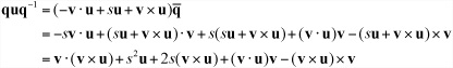
By the identities of the dot and cross products, the first term is zero and the last term is |v|2 – u(v · u)v, so you have
quq–1 =(s2—|v|2) u + 2s(v×u)+ 2(v · u)v
If you say t = |v| and set a to the normalized vector v/t, then you can rewrite this as
This represents a rotation about the axis a, with an angle θ given by cosθ – s2 = t2, sin θ = 2st, and 1 – cos θ = 2t2. Of these, you need only the last, since the first two together confirm that 1 – cosθ = 2t2, which you know because q is of unit length. The last is equivalent to saying that s2 + t2 = 1, which implies that ![]() . You can sum all this up by saying that a rotation around an axis a with angle θ can be calculated as follows using the quaternion:
. You can sum all this up by saying that a rotation around an axis a with angle θ can be calculated as follows using the quaternion:
This is a fairly significant improvement on the matrix form. One reason is that far fewer calculations are involved in the transformation. Another reason is that it’s much easier to see the relationship between the rotation and the quaternion than it is with the matrix. Also, just as with matrices, you can interpolate between two quaternions by taking a linear combination of them, although the rate at which the interpolation occurs is not the same as the rate at which the angle varies.
In addition to combining transforms to move objects from one place to another, you can use them to define relationships between different nodes. This allows you to move whole groups of nodes together by varying a single transform, just as varying a node’s transform can affect all the vertices of its model mesh.
You arrange all the nodes of the 3-D world in the form of a tree. In the tree, each node has exactly one parent and any number of children. The topmost node is the world itself, and each of the world node’s children has its own transform relative to the world. But the transform of a child node is applied relative to its parent. In other words, if the child’s relative transform is C and the parent’s transform is P, then the child’s transform relative to the world’s coordinate system is CP.
For example, suppose one model is sitting in the world with a world transform consisting of a rotation about the x-axis and a uniform scale. Any child of this model will be rotated and scaled before its own transform is applied. As a result, the model and its children act as a group. If the parent model is translated, rotated or scaled, its children, grandchildren, and so on will move along with it.
Note
In this section, what applies to translation in most cases can be applied to rotation and scaling.
Such movement means that there is a potential ambiguity when transforming an object. Say that you want to move an object 5 units along the z-axis. Which z-axis does that mean? It could be the node’s “local” z-axis, or its z-axis relative to its parent. It could also be the actual z-axis of the world. Figure 18.4 illustrates this situation.

Figure 18.4 represents a model of a car. The parent of the car is a ship on which the car is sitting. The car was modeled with its z-axis pointing along the body of the car. If you want to translate the car by 5 units along a z-axis, this could mean any of the directions indicated. The first is the car’s own z-axis, which is pointing along the world vector (1 0 1)T. The second is the ship’s z-axis, which is pointing along the world’s x-axis. The third is the world’s z-axis. Ultimately, you might want to use the z-axis of any other node in the scene.
Fortunately, each of these is easy to calculate. The z-axis of the node is given by the last column of its complete world transform matrix. In general, any direction vector can be found simply by transforming it with the node’s world transform. Similarly, while with a little work you can determine the direction of the parent’s z-axis or any other model’s, working out the world’s z-axis is even easier.
Commonly, you want to go the other way around. You need to know how to change the node’s personal transform in order to make it move along a particular vector. In this case, the simplest situation involves transforming the object in its local reference frame. Transforming locally is a matter of altering the transform of the object.
To alter the transform relative to the object’s parent’s transform is a little harder. To understand how this is so, suppose you want to move the object 5 pixels relative to the parent’s z-axis. You must first calculate the vector in the child’s reference frame. Expressed differently, you need a vector v such that Cv = k, which is given by v = C–1k. In English, this means that the vector v, when “untransformed” into parent-space, is equal to the z-vector k. Notice that this is the same independent of the parent’s own transform. Similarly, to translate relative to a world-vector, you must invert the complete world transform of the child node.
Note
The vector v does not need to be of unit length, since any of the transforms involved may include a scaling element. Actually, this is convenient, for it means you can perform your translation of 5 units without worrying about scale. To do so, you multiply by the already scaled vector v. But for rotations you need to remember to normalize the axis vector before performing the rotation.
Create functions that will apply a translation, scale, or rotation for a particular node relative to the world, the node’s parent, or the node itself. You should think about which method of storing transform information is most useful: as a single matrix or as three transformation vectors? Using quaternions for rotations?
In this chapter you have seen how homogeneous coordinates and mathematical gizmos like quaternions can be used to create a simple representation of a node’s disposition in 3-D space. In the process, you’ve also learned how to create smooth motion incorporating simultaneous rotation, translation, and scale transformations by interpolating between transforms.
In the next chapter, you’ll take one final look at collision detection by extending your previous work into the third dimension.
The meaning of the term transform and how it is represented in various forms: as a single matrix, as a combination of separate matrices, and as three vectors
How quaternions can be used to create a simpler representation of rotations
How transforms can be combined to move objects from place to place, and to create groups of objects with a fixed position relative to one another