
Given that the frontend of the JIT compiler is finished with the bytecode, having turned it into some other form that is easier to process, what happens next? Typically, the code goes through several levels of transformations and optimizations, each level becoming increasingly platform-dependent. The final level of code is native code for a particular platform. The native code is emitted into a code buffer and executed whenever the function it represents is called.
Naturally, it makes sense to keep the JIT compiler portable as far as possible. So, most optimizations are usually done when the intermediate code format is still platform-independent. This makes it easier to port the JIT compiler to different architectures. However, low-level, platform-specific optimizations must naturally be implemented as well to achieve industrial strength performance.
This section describes how the JIT compiler gets from bytecode to native code and the stages involved. We concentrate on the JRockit JIT compiler, but in general terms the process of generating native code is similar between JVMs.
JRockit uses the code generation strategy total JIT compilation.
When the JRockit project started in 1998, the JVM architects realized early on that pure server-side Java was a niche so far unexploited, and JRockit was originally designed to be only a server-side JVM. Most server-side applications, it was argued, stay running for a long time and can afford to take some time reaching a steady state. Thus, for a server-side-only JVM, it was decided that code generation time was a smaller problem than efficient execution. This saved us the trouble of implementing both a JIT compiler and a bytecode interpreter as well as handling the state transitions between them.
It was quickly noted that compiling every method contributed to additional startup time. This was initially not considered to be a major issue. Server-side applications, once they are up and running, stay running for a long time.
Later, as JRockit became a major mainstream JVM, known for its performance, the need to diversify the code pipeline into client and server parts was recognized. No interpreter was added, however. Rather the JIT was modified to differentiate even further between cold and hot code, enabling faster "sloppy" code generation the first time a method was encountered. This greatly improved startup time to a satisfying degree, but of course, getting to pure interpreter speeds with a compile-only approach is still very hard.
Another aspect that makes life easier with an interpreter is debuggability. Bytecode contains meta information about things like variable names and line numbers. These are needed by the debugger. In order to support debuggability, the JRockit JIT had to propagate this kind of information all the way from per-bytecode basis to per-native instruction basis. Once that bookkeeping problem was solved, there was little reason to add an interpreter. This has the added benefit that, to our knowledge, JRockit is the only virtual machine that lets the user debug optimized code.
The main problems with the compile-only strategy in JRockit are the code bloat (solved by garbage collecting code buffers with methods no longer in use) and compilation time for large methods (solved by having a sloppy mode for the JIT).
Note
The compile-only strategy is sometimes less scalable than it should be. For example, sometimes, JRockit will use a lot of time generating a relatively large method, the typical example being a JSP. Once finished, however, the response time for accessing that JSP will be better than that of an interpreted version.
If you run into problems with code generation time using JRockit, these can often be worked around. More on this will be covered in the Controlling code generation in JRockit section at the end of this chapter.
The "brain" of the JRockit JVM is the runtime system itself. It keeps track of what goes on in the world that comprises the virtual execution environment. The runtime system is aware of which Java classes and methods make up the "world" and requests that the code generator compiles them at appropriate times with appropriate levels of code quality.
To simplify things a bit, the first thing the runtime wants to do when the JVM is started, is to look up and jump to the main method of a Java program. This is done through a standard JNI call from the native JVM, just like any other native application would use JNI to call Java code.
Searching for main triggers a complex chain of actions and dependencies. A lot of other Java methods required for bootstrapping and fundamental JVM behavior need to be generated in order to resolve the main function. When finally main is ready and compiled to native code, the JVM can execute its first native-to-Java stub and pass control from the JVM to the Java program.
Note
To study the bootstrap behavior of JRockit, try running a simple Java program with the command-line switch -Xverbose:codegen. It may seem shocking that running a simple "Hello World" program involves JIT compiling around 1,000 methods. This, however, takes very little time. On a modern Intel Core2 machine, the total code generation time is less than 250 milliseconds.
Total JIT compilation needs to be a lazy process. If any method or class referenced from another method would be fully generated depth first at referral time, there would be significant code generation overhead. Also, just because a class is referenced from the code doesn't mean that every method of the class has to be compiled right away or even that any of its methods will ever be executed. Control flow through the Java program might take a different path. This problem obviously doesn't exist in a mixed mode solution, in which everything starts out as interpreted bytecode with no need to compile ahead of execution.
JRockit solves this problem by generating stub code for newly referred but not yet generated methods. These stubs are called trampolines, and basically consist of a few lines of native code pretending to be the final version of the method. When the method is first called, and control jumps to the trampoline, all it does is execute a call that tells JRockit that the real method needs to be generated. The code generator fulfils the request and returns the starting address of the real method, to which the trampoline then dispatches control. To the user it looks like the Java method was called directly, when in fact it was generated just at the first time it was actually called.
0x1000: method A
call method B @ 0x2000
|
0x3000: method C
call method B @ 0x2000
|
0x2000: method B (trampoline) call JVM.Generate(B) -> start write trap @ 0x2000 goto start @ 0x4000 |
0x4000: The "real" method B ... |
Consider the previous example. method A, whose generated code resides at address 0x1000 is executing a call to method B, that it believes is placed at address 0x2000. This is the first call to method B ever. Consequently, all that is at address 0x2000 is a trampoline. The first thing the trampoline does is to issue a native call to the JVM, telling it to generate the real method B. Execution then halts until this code generation request has been fulfilled, and a starting address for method B is returned, let's say 0x4000. The trampoline then dispatches control to method B by jumping to that address.
Note that there may be several calls to method B in the code already, also pointing to the trampoline address 0x2000. Consider, for example, the call in method C that hasn't been executed yet. These calls need to be updated as well, without method B being regenerated. JRockit solves this by writing an illegal instruction at address 0x2000, when the trampoline has run. This way, the system will trap if the trampoline is called more than once. The JVM has a special exception handler that catches the trap, and patches the call to the trampoline so that it points to the real method instead. In this case it means overwriting the call to 0x2000 in method C with a call to 0x4000. This process is called back patching.
Back patching is used for all kinds of code replacement in the virtual machine, not just for method generation. If, for example, a hot method has been regenerated to a more efficient version, the cold version of the code is fitted with a trap at the start and back patching takes place in a similar manner, gradually redirecting calls from the old method to the new one.
Again, note that this is a lazy approach. We don't have time to go over the entire compiled code base and look for potential jumps to code that has changed since the caller was generated.
If there are no more references to an older version of a method, its native code buffer can be scheduled for garbage collection by the run time system so as to unclutter the memory. This is necessary in a world that uses a total JIT strategy because the amount of code produced can be quite large.
In JRockit, code generation requests are passed to the code generator from the runtime when a method needs to be compiled. The requests can be either synchronous or asynchronous.
Synchronous code generation requests do one of the following:
- Quickly generate a method for the JIT, with a specified level of efficiency
- Generate an optimized method, with a specified level of efficiency
An asynchronous request is:
- Act upon an invalidated assumption, for example, force regeneration of a method or patch the native code of a method
Internally, JRockit keeps synchronous code generation requests in a code generation queue and an optimization queue, depending on request type. The queues are consumed by one or more code generation and/or optimization threads, depending on system configuration.
The code generation queue contains generation requests for methods that are needed for program execution to proceed. These requests, except for special cases during bootstrapping, are essentially generated by trampolines. The call "generate me" that each trampoline contains, inserts a request in the code generation queue, and blocks until the method generation is complete. The return value of the call is the address in memory where the new method starts, to which the trampoline finally jumps.
Optimization requests are added to the optimization queue whenever a method is found to be hot, that is when the runtime system has realized that we are spending enough time executing the Java code of that method so that optimization is warranted.
The optimization queue understandably runs at a lower priority than the code generation queue as its work is not necessary for code execution, but just for code performance. Also, an optimization request usually takes orders of magnitude longer than a standard code generation request to execute, trading compile time for efficient code.
Once an optimized version of a method is generated, the existing version of the code for that method needs to be replaced. As previously described, the method entry point of the existing cold version of the method is overwritten with a trap instruction. Calls to the old method will be back patched to point to the new, optimized piece of code.
If the Java program spends a very large amount of time in a method, it will be flagged as hot and queued for replacement. However, consider the case where the method contains a loop that executes for a very long time. This method may well be hotspotted and regenerated, but the old method still keeps executing even if the method entry to the old method is fitted with a trap. Obviously, the performance enhancement that the optimized method contributes will enter the runtime much later, or never if the loop is infinite.
Some optimizers swap out code on the existing execution stack by replacing the code of a method with a new version in the middle of its execution. This is referred to as on-stack replacement and requires extensive bookkeeping. Though this is possible in a completely JIT-compiled world, it is easier to implement where there is an interpreter to fall back to.
JRockit doesn't do on-stack replacement, as the complexity required to do so is deemed too great. Even though the code for a more optimal version of the method may have been generated, JRockit will continue executing the old version of the method if it is currently running.
Our research has shown that in the real world, this matters little for achieving performance. The only places we have encountered performance penalties because of not doing on-stack replacement is in badly written micro benchmarks, such as when the main function contains all the computations in a very long loop. Moving the bulk of the benchmark into a separate function and calling this repeatedly from main will resolve this problem. We will thoroughly discuss the most important aspects of benchmarking in Chapter 5.
The code generator in the JVM has to perform a number of necessary bookkeeping tasks for the runtime system.
For various reasons, a garbage collector needs to keep track of which registers and stack frame locations contain Java objects at any given point in the program. This information is generated by the JIT compiler and is stored in a database in the runtime system. The JIT compiler is the component responsible for creating this data because type information is available "for free" while generating code. The compiler has to deal with types anyway. In JRockit, the object meta info is called livemaps, and a detailed explanation of how the code generation system works with the garbage collector is given in Chapter 3, Adaptive Memory Management.
Another bookkeeping issue in the compiled world is the challenge of preserving source code level information all the way down to machine language. The JVM must always be able to trace program points back from an arbitrary native instruction to a particular line of Java source code. We need to support proper stack traces for debugging purposes, even stack traces containing optimized code. This gets even more complicated as the optimizer may have transformed a method heavily from its original form. A method may even contain parts of other methods due to inlining. If an exception occurs anywhere in our highly optimized native code, the stack trace must still be able to show the line number where this happened.
This is not a difficult problem to solve—bookkeeping just involves some kind of database, as it is large and complex. JRockit successfully preserves mappings between most native instructions and the actual line of Java source code that created them. This, obviously, is much more work in a compiled world than in an interpreted one. In the Java bytecode format, local variable information and line number information are mapped to individual bytecodes, but JRockit has to make sure that the mapping survives all the way down to native code. Each bytecode instruction eventually turns into zero or more native code instructions that may or may not execute in sequence.
Finally, as we have already discussed, remembering what assumptions or "gambles" have been made while generating methods is vital in Java. As soon as one of the assumptions is violated, we need to send asynchronous code regeneration requests for whatever methods are affected. Thus, an assumption database is another part of the JRockit runtime that communicates with the code generator.
Let us now take a look at what happens on the road from bytecode to native code in the JRockit JIT compiler. This section describes how a small method is transformed to native code by the JRockit JIT. Large parts of this process are similar in other JIT compilers (as well as in other static compilers), and some parts are not. The end result, native code, is the same.
Let us, consider the following Java method as an example:
public static int md5_F(int x, int y, int z) {
return (x & y) | ((~x) & z);
}
This is part of the well known MD5 hash function and performs bit operations on three pieces of input.
The first stage of the JRockit code pipeline turns the bytecode into an Intermediate Representation (IR). As it is conceivable that other languages may be compiled by the same frontend, and also for convenience, optimizers tend to work with a common internal intermediate format.
JRockit works with an intermediate format that differs from bytecode, looking more like classic text book compiler formats. This is the common approach that most compilers use, but of course the format of IR that a compiler uses always varies slightly depending on implementation and the language being compiled.
Aside from the previously mentioned portability issue, JRockit also doesn't work with bytecode internally because of the issues with unstructured control flow and the execution stack model, which differs from any modern hardware register model.
Because we lack the information to completely reconstruct the ASTs, a method in JRockit is represented as a directed graph, a control flow graph, whose nodes are basic blocks. The definition of a basic block is that if one instruction in the basic block is executed, all other instructions in it will be executed as well. Since there are no branches in our example, the md5_F function will turn into exactly one basic block.
A basic block contains zero to many operations, which in turn have operands. Operands can be other operations (forming expression trees), variables (virtual registers or atomic operands), constants, addresses, and so on, depending on how close to the actual hardware representation the IR is.
Basic blocks can have multiple entries and multiple exits. The edges in the graph represent control flow. Any control flow construct, such as a simple fallthrough to the next basic block, a goto, a conditional jump, a switch, or an exception, produces one or more edges in the graph.
When control enters a method, there is a designated start basic block for the execution. A basic block with no exits ends the method execution. Typically such a block ends with a return or throw clause.
A small complication is the presence of exceptions, which, if consistent to this model, should form conditional jumps from every bytecode operation that may fault to an appropriate catch block, where one is available.
This would quickly turn into a combinatorial explosion of edges in the flow graph (and consequently of basic blocks), severely handicapping any O(|V||E|) (nodes x edges) graph traversal algorithm that needs to work on the code. Therefore, exceptions are treated specially on a per-basic block basis instead.
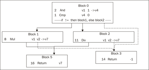
This figure shows the basic block graph of a slightly larger example. Method entry is at Block 0 that has three exits—two normal ones, as it contains a conditional branch, and an exception edge. This means that Block 0 is a try block, whose catch starts at Block 3. The same try block spans Block 1 and Block 2 as well. The method can exit either by triggering the exception and ending up in Block 3 or by falling through to Block 5. Both these blocks end with return instructions. Even though the only instruction that can trigger an exception is the div in Block 2 (on division by zero), the try block spans several nodes because this is what the bytecode (and possibly the source code) looked like. Optimizers may choose to deal with this later.
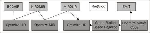
This following figure illustrates the different stages of the JRockit code pipeline:

The first module in the code generator, BC2HIR, is the frontend against the bytecode and its purpose is to quickly translate bytecodes into IR. HIR in this case stands for High-level Intermediate Representation. For the md5_F method, where no control flow in the form of conditional or unconditional jumps is present, we get just one basic block.
The following code snippet shows the md5_F method in bytecode form:
public static int md5_F(int, int, int);
Code: Stack contents: Emitted code:
0: iload_0 v0
1: iload_1 v1
2: iand (v0&v1)
3: iload_0 (v0&v1), v0
4: iconst_m1 (v0&v1), v0, -1
5: ixor (v0&v1), (v0^-1)
6: iload_2 (v0&v1), (v0^-1), v2
7: iand (v0&v1), ((v0^-1) & v2)
8: ior ((v0&v1) | ((v0^-1) & v2))
9: ireturn return ((v0&v1) | ((v0^-1) & v2));
The JIT works by computing a control flow graph for the IR by examining where the jumps in the bytecode are, and then filling its basic blocks with code. Code is constructed by emulating the contents of the evaluation stack at any given location in the program. Emulating a bytecode operation results in changes to the evaluation stack and/or code being generated. The example has been annotated with the contents of the emulated evaluation stack and the resulting generated code after each bytecode has been processed
Note
Bit negation (~) is implemented by javac as an xor with -1 (0xffffffff), as bytecode lacks a specific not operator.
As we can see, by representing the contents of a variable on the evaluation stack with a variable handle, we can reconstruct the expressions from the original source code. For example, the iload_0 instruction, which means "push the contents of variable 0" turns into the expression "variable 0" on the emulated stack. In the example, the emulator gradually forms a more and more complex expression on the stack, and when it is time to pop it and return it, the expression in its entirety can be used to form code.
This is the output, the High-level IR, or HIR:
Note
In JRockit IR, the annotation @ before each statement identifies its program point in the code all the way down to assembler level. The first number following the @ is the bytecode offset of the expression and the last is the source code line number information. This is part of the complex meta info framework in JRockit that maps individual native instructions back to their Java program points.
The variable indexes were assigned by JRockit, and differ from those in the bytecode. Notice that operations may contain other operations as their operands, similar to the original Java code. These nested expressions are actually a useful byproduct of turning the bytecode stack back into expressions. This way we get a High-level Representation instead of typical "flat" compiler code with temporary variable assignments, where operations may not contain other operations. The HIR lends itself well to some optimizations that are harder to do on another format; for example, discovering if a sub-expression (in the form of a subtree) is present twice in an expression. Then the sub-expression can be folded into a temporary variable, saving it from being evaluated twice.
Emulating the bytecode stack to form HIR is not without problems though. Since at compile time, we only know what expression is on the stack, and not its value, we run into various problems. One example would be in situations where the stack is used as memory. Take for example the construct result = x ? a : b. The bytecode compiles into something like this:
/* bytecode for: "return x ? a : b" */
static int test(boolean x, int a, int b);
0: iload_0 //push x
1: ifeq 8 //if x == false then goto 8
4: iload_1 //push a
5: goto 9
8: iload_2 //push b
9: ireturn //return pop
When the emulator gets to the ireturn instruction, the value popped can be either a (local variable 1) or b (local variable 2). Since we can't express "either a or b" as a variable, we need to replace the loads at offsets 4 and 8 with writes to one and the same temporary variable, and place that on the stack instead.
The BC2HIR module that turns bytecodes into a control flow graph with expressions is not computationally complex. However, it contains several other little special cases, similar to the earlier one, which are beyond the scope of this book. Most of them have to do with the lack of structure in byte code and with the evaluation stack metaphor. Another example would be the need to associate monitorenter bytecodes with their corresponding monitorexit(s), the need for which is explained in great detail in Chapter 4.
MIR or Middle-level Intermediate Representation, is the transform domain where most code optimizations take place. This is because most optimizations work best with three address code or rather instructions that only contain atomic operands, not other instructions. Transforming HIR to MIR is simply an in-order traversal of the expression trees mentioned earlier and the creation of temporary variables. As no hardware deals with expression trees, it is natural that code turns into progressively simpler operations on the path through the code pipeline.
Our md5_F example would look something like the following code to the JIT compiler, when the expression trees have been flattened. Note that no operation contains other operations anymore. Each operation writes its result to a temporary variable, which is in turn used by later operations.
params: v1 v2 v3
block0: [first] [id=0]
2 @2:49* (i32) and v1 v2 -> v4
5 @5:49* (i32) xor v1 -1 -> v5
7 @7:49* (i32) and v5 v3 -> v5
8 @8:49* (i32) or v4 v5 -> v4
10 @9:49* (i32) return v4
If the JIT compiler is executing a code generation request from the optimizer, most optimizations on the way down to native code are carried out on MIR. This will be discussed later in the chapter.
After MIR, it is time to turn platform dependent as we are approaching native code. LIR, or Low-level IR, looks different depending on hardware architecture.
Consider the Intel x86, where the biggest customer base for JRockit exists. The x86 has legacy operations dating back to the early 1980s. The RISC-like format of the previous MIR operations is inappropriate. For example, a logical and operation on the x86 requires the same first source and destination operand. That is why we need to introduce a number of new temporaries in order to turn the code into something that fits the x86 model better.
If we were compiling for SPARC, whose native format looks more like the JRockit IR, fewer transformations would have been needed.
Following is the LIR for the md5_F method on a 32-bit x86 platform:
params: v1 v2 v3
block0: [first] [id=0]
2 @2:49* (i32) x86_and v2 v1 -> v2
11 @2:49 (i32) x86_mov v2 -> v4
5 @5:49* (i32) x86_xor v1 -1 -> v1
12 @5:49 (i32) x86_mov v1 -> v5
7 @7:49* (i32) x86_and v5 v3 -> v5
8 @8:49* (i32) x86_or v4 v5 -> v4
14 @9:49 (i32) x86_mov v4 -> eax
13 @9:49* (i32) x86_ret eax
A couple of platform-independent mov instructions have been inserted to get the correct x86 semantics. Note that the and, xor, and or operations now have the same first operand as destination, the way x86 requires. Another interesting thing is that we already see hard-coded machine registers here. The JRockit calling convention demands that integers be returned in the register eax, so the register allocator that is the next step of the code pipeline doesn't really have a choice for a register for the return value.
There can be any number of virtual registers (variables) in the code, but the physical platform only has a small number of them. Therefore, the JIT compiler needs to do register allocation, transforming the virtual variable mappings into machine registers. If at any given point in the program, we need to use more variables than there are physical registers in the machine at the same time, the local stack frame has to be used for temporary storage. This is called spilling, and the register allocator implements spills by inserting move instructions that shuffle registers back and forth from the stack. Naturally spill moves incur overhead, so their placement is highly significant in optimized code.
Register allocation is a very fast process if done sloppily, such as in the first JIT stage, but computationally intensive if a good job is needed, especially when there are many variables in use (or live) at the same time. However, because of the small number of variables, we get an optimal result with little effort in our example method. Several of the temporary mov instructions have been coalesced and removed.
Our md5_F method needs no spills, as x86 has seven available registers (15 on the 64-bit platforms), and we use only three.
params: ecx eax edx
block0: [first] [id=0]
2 @2:49* (i32) x86_and eax ecx -> eax
5 @5:49* (i32) x86_xor ecx -1 -> ecx
7 @7:49* (i32) x86_and ecx edx -> ecx
8 @8:49* (i32) x86_or eax ecx -> eax
13 @9:49* (void) x86_ret eax
Every instruction in our register allocated LIR has a native instruction equivalent on the platform that we are generating code for.
Just to put spill code in to perspective, following is a slightly longer example. The main method of the Spill program does eight field loads to eight variables that are then used at the same time (for multiplying them together).
public class Spill {
static int aField, bField, cField, dField;
static int eField, fField, gField, hField;
static int answer;
public static void main(String args[]) {
int a = aField;
int b = bField;
int c = cField;
int d = dField;
int e = eField;
int f = fField;
int g = gField;
int h = hField;
answer = a*b*c*d*e*f*g*h;
}
}
We will examine the native code for this method on a 32-bit x86 platform. As 32-bit x86 has only seven available registers, one of the intermediate values has to be spilled to the stack. The resulting register allocated LIR code is shown in the following code snippet:
Note
Assembly or LIR instructions that dereference memory typically annotate their pointers as a value or variable within square brackets. For example, [esp+8] dereferences the memory eight bytes above the stack pointer (esp) on x86 architectures.
block0: [first] [id=0]
68 (i32) x86_push ebx //store callee save reg
69 (i32) x86_push ebp //store callee save reg
70 (i32) x86_sub esp 4 -> esp //alloc stack for 1 spill
43 @0:7* (i32) x86_mov [0xf56bd7f8] -> esi //*aField->esi (a)
44 @4:8* (i32) x86_mov [0xf56bd7fc] -> edx //*bField->edx (b)
67 @4:8 (i32) x86_mov edx -> [esp+0x0] //spill b to stack
45 @8:9* (i32) x86_mov [0xf56bd800] -> edi //*cField->edi (c)
46 @12:10* (i32) x86_mov [0xf56bd804] -> ecx //*dField->ecx (d)
47 @17:11* (i32) x86_mov [0xf56bd808] -> edx //*eField->edx (e)
48 @22:12* (i32) x86_mov [0xf56bd80c] -> eax //*fField->eax (f)
49 @27:13* (i32) x86_mov [0xf56bd810] -> ebx //*gField->ebx (g)
50 @32:14* (i32) x86_mov [0xf56bd814] -> ebp //*hField->ebp (h)
26 @39:16 (i32) x86_imul esi [esp+0x0] -> esi //a *= b
28 @41:16 (i32) x86_imul esi edi -> esi //a *= c
30 @44:16 (i32) x86_imul esi ecx -> esi //a *= d
32 @47:16 (i32) x86_imul esi edx -> esi //a *= e
34 @50:16 (i32) x86_imul esi eax -> esi //a *= f
36 @53:16 (i32) x86_imul esi ebx -> esi //a *= g
38 @56:16 (i32) x86_imul esi ebp -> esi //a *= h
65 @57:16* (i32) x86_mov esi -> [0xf56bd818] //*answer = a
71 @60:18* (i32) x86_add esp, 4 -> esp //free stack slot
72 @60:18 (i32) x86_pop -> ebp //restore used callee save
73 @60:18 (i32) x86_pop -> ebx //restore used callee save
66 @60:18 (void) x86_ret //return
We can also note that the register allocator has added an epilogue and prologue to the method in which stack manipulation takes place. This is because it has figured out that one stack position will be required for the spilled variable and that it also needs to use two callee-save registers for storage. A register being callee-save means that a called method has to preserve the contents of the register for the caller. If the method needs to overwrite callee-save registers, they have to be stored on the local stack frame and restored just before the method returns. By JRockit convention on x86, callee-save registers for Java code are ebx and ebp. Any calling convention typically includes a few callee-save registers since if every register was potentially destroyed over a call, the end result would be even more spill code.
After register allocation, every operation in the IR maps one-to-one to a native operation in x86 machine language and we can send the IR to the code emitter. The last thing that the JIT compiler does to the register allocated LIR is to add mov instructions for parameter marshalling (in this case moving values from in-parameters as defined by the calling convention to positions that the register allocator has picked). Even though the register allocator thought it appropriate to put the first parameter in ecx, compilers work internally with a predefined calling convention. JRockit passes the first parameter in eax instead, requiring a shuffle mov. In the example, the JRockit calling convention passes parameters x in eax, y in edx, and z in esi respectively.
Note
Assembly code displayed in figures generated by code dumps from JRockit use Intel style syntax on the x86, with the destination as the first operand, for example "and ebx, eax" means "ebx = ebx & eax".
Following is the resulting native code in a code buffer:
[method is md5_F(III)I [02DB2FF0 - 02DB3002]]
02DB2FF0: mov ecx,eax
02DB2FF2: mov eax,edx
02DB2FF4: and eax,ecx
02DB2FF6: xor ecx,0xffffffff
02DB2FF9: and ecx,esi
02DB2FFC: or eax,ecx
02DB2FFF: ret
Regenerating an optimized version of a method found to be hot is not too dissimilar to normal JIT compilation. The optimizing JIT compiler basically piggybacks on the original code pipeline, using it as a "spine" for the code generation process, but at each stage, an optimization module is plugged into the JIT.
Different optimizations are suitable for different levels of IR. For example, HIR lends itself well to value numbering in expression trees, substituting two equivalent subtrees of an expression with one subtree and a temporary variable assignment.
MIR readily transforms into Single Static Assignment (SSA) form, a transform domain that makes sure that any variable has only one definition. SSA transformation is part of virtually every commercial compiler today and makes implementing many code optimizations much easier. Another added benefit is that code optimizations in SSA form can be potentially more powerful.
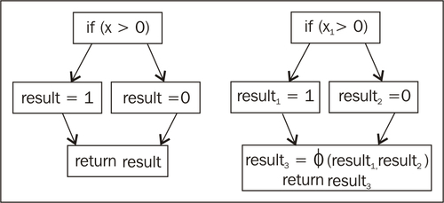
The previous flow graph shows what happens before and after transformation to SSA form. The result variable that is returned by the program is assigned either 1 or 0 depending on the value of x and the branch destination. Since SSA form allows only one assignment of each variable, the result variable has been split into three different variables. At the return statement, result can either be result1 or result2. To express this "either" semantic, a special join operator, denoted by the Greek letter phi (Φ), is used. Trivially, no hardware platform can express this ambiguity, so the code has to be transformed back to normal form before emission. The reverse transform basically replaces each join operator with preceding assignments, one per flow path, to the destination of the join instruction.
Many classic code optimizations such as constant propagation and copy propagation have their own faster SSA form equivalents. This mostly has to do with the fact that given any use of a variable, it is unambiguous where in the code that variable is defined. There is plenty of literature on the subject and a thorough discussion on all the benefits of SSA form is beyond the scope of this book.
LIR is platform-dependent and initially not register allocated, so transformations that form more efficient native operation sequences can be performed here. An example would be replacing dumb copy loops with specialized Intel SSE4 instructions for faster array copies on the x86.
Note
When generating optimized code, register allocation tends to be very important. Any compiler textbook will tell you that optimal register allocation basically is the same problem as graph coloring. This is because if two variables are in use at the same time, they obviously cannot share the same register. Variables in use at the same time can be represented as connected nodes in a graph. The problem of register allocation can then be reduced to assigning colors to the nodes in the graph, so that no connected nodes have the same color. The amount of colors available is the same as the number of registers on the platform. Sadly enough, in computational complexity terms, graph coloring is NP-hard. This means that no efficient (polynomial time) algorithm exists that can solve the problem. However, graph coloring can be approximated in quadratic time. Most compilers contain some variant of the graph coloring algorithm for register allocation.
The JRockit optimizer contains a very advanced register allocator that is based on a technique called graph fusion, that extends the standard graph coloring approximation algorithm to work on subregions in the IR. Graph fusion has the attractive property that the edges in the flow graph, processed early, generate fewer spills than the edges processed later. Therefore, if we can pick hot subregions before cold ones, the resulting code will be more optimal. Additional penalty comes from the need to insert shuffle code when fusing regions in order to form a complete method. Shuffle code consists of sequences of move instructions to copy the contents of one local register allocation into another one.
Finally, just before code emission, various peephole optimizations can be applied to the native code, replacing one to several register allocated instructions in sequence with more optimal ones.
Note
Clearing a register is usually done by XORing the register with itself. Replacing instructions such as mov eax, 0 with xor eax, eax, which is potentially faster, is an example of a peephole optimization that works on exactly one instruction. Another example would be turning a multiplication with the power of two followed by an add instruction into a simple lea instruction on x86, optimized to do both.
A complete walkthrough of the JRockit code pipeline with the algorithms and optimizations within would be the subject for an entire book of its own. This section merely tries to highlight some of the things that a JVM can do with code, given adequate runtime feedback.
Generating optimized code for a method in JRockit generally takes 10 to 100 times as long as JITing it with no demands for execution speed. Therefore, it is important to only optimize frequently executed methods.
Grossly oversimplifying things, the bulk of the optimizer modules plugged into the code pipeline work like this:
do {
1) get rid of calls, exposing more control flow through aggressive inlining.
2) apply optimizations on enlarged code mass, try to shrink it.
} while ("enough time left" && "code not growing too fast");
Java is an object-oriented language and contains a lot of getters, setters, and other small "nuisance" calls. The compiler has to presume that calls do very complex things and have side effects unless it knows what's inside them. So, for simplification, small methods are frequently inlined, replacing the call with the code of the called function. JRockit tries to aggressively inline everything that seems remotely interesting on hot execution paths, with reasonable prioritization of candidates using sample and profiling information.
In a statically compiled environment, too aggressive inlining would be total overkill, and too large methods would cause instruction cache penalties and slow down execution. In a runtime, however, we can hope to have good enough sample information to make more realistic guesses about what needs to be inlined.
After bringing in whatever good inlining candidates we can find into the method, the JIT applies optimizations to the, now usually quite large, code mass, trying to shrink it. For example, this is done by folding constants, eliminating expressions based on escape analysis, and applying plenty of other simplifying transforms. Dead code that is proved never to be executed is removed. Multiple loads and stores that access the same memory location can, under certain conditions, be eliminated, and so on.
Surprisingly enough, the size of the total code mass after inlining and then optimizing the inlined code is often less than the original code mass of a method before anything was inlined.
The runtime system can perform relatively large simplifications, given relatively little input. Consider the following program that implements the representation of a circle by its radius and allows for area computation:
public class Circle {
private double radius;
public Circle(int radius) {
this.radius = radius;
}
public double getArea() {
return 3.1415 * radius * radius;
}
public static double getAreaFromRadius(int radius) {
Circle c = new Circle(radius);
return c.getArea();
}
static int areas[] = new int[0x10000];
static int radii[] = new int[0x10000];
static java.util.Random r = new java.util.Random();
static int MAX_ITERATIONS = 1000;
public static void gen() {
for (int i = 0; i < areas.length; i++) {
areas[i] = (int)getAreaFromRadius(radii[i]);
}
}
public static void main(String args[]) {
for (int i = 0; i < radii.length; i++) {
radii[i] = r.nextInt();
}
for (int i = 0; i < MAX_ITERATIONS; i++) {
gen(); //avoid on stack replacement problems
}
}
}
Running the previous program with JRockit with the command-line flag -Xverbose:opt,gc, to make JRockit dump all garbage collection and code optimization events, produces the following output:
hastur:material marcus$ java Xverbose:opt,gc Circle
[INFO ][memory ] [YC#1] 0.584-0.587: YC 33280KB->8962KB (65536KB), 0.003 s, sum of pauses 2.546 ms, longest pause 2.546 ms
[INFO ][memory ] [YC#2] 0.665-0.666: YC 33536KB->9026KB (65536KB), 0.001 s, sum of pauses 0.533 ms, longest pause 0.533 ms
[INFO ][memory ] [YC#3] 0.743-0.743: YC 33600KB->9026KB (65536KB), 0.001 s, sum of pauses 0.462 ms, longest pause 0.462 ms
[INFO ][memory ] [YC#4] 0.821-0.821: YC 33600KB->9026KB (65536KB), 0.001 s, sum of pauses 0.462 ms, longest pause 0.462 ms
[INFO ][memory ] [YC#5] 0.898-0.899: YC 33600KB->9026KB (65536KB), 0.001 s, sum of pauses 0.463 ms, longest pause 0.463 ms
[INFO ][memory ] [YC#6] 0.975-0.976: YC 33600KB->9026KB (65536KB), 0.001 s, sum of pauses 0.448 ms, longest pause 0.448 ms
[INFO ][memory ] [YC#7] 1.055-1.055: YC 33600KB->9026KB (65536KB), 0.001 s, sum of pauses 0.461 ms, longest pause 0.461 ms
[INFO ][memory ] [YC#8] 1.132-1.133: YC 33600KB->9026KB (65536KB), 0.001 s, sum of pauses 0.448 ms, longest pause 0.448 ms
[INFO ][memory ] [YC#9] 1.210-1.210: YC 33600KB->9026KB (65536KB), 0.001 s, sum of pauses 0.480 ms, longest pause 0.480 ms
[INFO ][opt ][00020] #1 (Opt) jrockit/vm/Allocator.allocObjectOrArray(IIIZ)Ljava/lang/Object;
[INFO ][opt ][00020] #1 1.575-1.581 0x9e04c000-0x9e04c1ad 5 .72 ms 192KB 49274 bc/s (5.72 ms 49274 bc/s)
[INFO ][memory ] [YC#10] 1.607-1.608: YC 33600KB->9090KB (65536KB), 0.001 s, sum of pauses 0.650 ms, longest pause 0.650 ms
[INFO ][memory ] [YC#11] 1.671-1.672: YC 33664KB->9090KB (65536KB), 0.001 s, sum of pauses 0.453 ms, longest pause 0.453 ms.
[INFO ][opt ][00020] #2 (Opt) jrockit/vm/Allocator.allocObject(I)Ljava/lang/Object;
optimized codeoptimized codeworking[INFO ][opt ][00020] #2 1.685-1.689 0x9e04c1c0-0x9e04c30d 3 .88 ms 192KB 83078 bc/s (9.60 ms 62923 bc/s)
[INFO ][memory ] [YC#12] 1.733-1.734: YC 33664KB->9090KB (65536KB), 0.001 s, sum of pauses 0.459 ms, longest pause 0.459 ms.
[INFO ][opt ][00020] #3 (Opt) Circle.gen()V
[INFO ][opt ][00020] #3 1.741-1.743 0x9e04c320-0x9e04c3f2 2 .43 ms 128KB 44937 bc/s (12.02 ms 59295 bc/s)
[INFO ][opt ][00020] #4 (Opt) Circle.main([Ljava/lang/String;)V
[INFO ][opt ][00020] #4 1.818-1.829 0x9e04c400-0x9e04c7af 11 .04 ms 384KB 27364 bc/s (23.06 ms 44013 bc/s)
hastur:material marcus$
No more output is produced until the program is finished.
The various log formats for the code generator will be discussed in more detail at the end of this chapter. Log formats for the memory manager are covered in Chapter 3.
It can be noticed here, except for optimization being performed on the four hottest methods in the code (where two are JRockit internal), that the garbage collections stop after the optimizations have completed. This is because the optimizer was able to prove that the Circle objects created in the getAreaFromRadius method aren't escaping from the scope of the method. They are only used for an area calculation. Once the call to c.getArea is inlined, it becomes clear that the entire lifecycle of the Circle objects is spent in the getAreaFromRadius method. A Circle object just contains a radius field, a single double, and is thus easily represented just as that double if we know it has a limited lifespan. An allocation that caused significant garbage collection overhead was removed by intelligent optimization.
Naturally, this is a fairly trivial example, and the optimization issue is easy for the programmer to avoid by not instantiating a Circle every time the area method is called in the first place. However, if properly implemented, adaptive optimizations scale well to large object-oriented applications.
Note
The runtime is always better than the programmer at detecting certain patterns. It is often surprising what optimization opportunities the virtual machine discovers, that a human programmer hasn't seen. It is equally surprising how rarely a "gamble", such as assuming that a particular method never will be overridden, is invalidated. This shows some of the true strength of the adaptive runtime.
Unoptimized Java carries plenty of overhead. The javac compiler needs to do workarounds to implement some language features in bytecode. For example, string concatenation with the + operator is just syntactic sugar for the creation of StringBuilder objects and calls to their append functions. An optimizing compiler should, however, have very few problems transforming things like this into more optimal constructs. For example, we can use the fact that the implementation of java.lang.StringBuilder is known, and tell the optimizer that its methods have no harmful side effects, even though they haven't been generated yet.
Similar issues exist with boxed types. Boxed types turn into hidden objects (for example instances of java.lang.Integer) on the bytecode level. Several traditional compiler optimizations, such as escape analysis, can often easily strip down a boxed type to its primitive value. This removes the hidden object allocation that javac put in the bytecode to implement the boxed type.