
Analyzing JRA recordings may easily seem like black magic to the uninitiated, so just like we did with the Management Console, we will go through each tab of the JRA editor to explain the information in that particular tab, with examples on when it is useful.
Just like in the console, there are several tabs in different tab groups.
The tabs in the General tab group provide views of key characteristics and recording metadata. In JRA, there are three tabs—Overview, Recording, and System.
The first tab in the General tab group is the Overview tab. This tab contains an overview of selected key information from the recording. The information is useful for checking the system health at a glance.
The first section in the tab is a dial dashboard that contains CPU usage, heap, and pause time statistics.
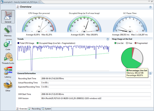
What to look for depends on the system. Ideally the system should be well utilized, but not saturated. A good rule of thumb for most setups would be to keep the Occupied Heap (Live Set + Fragmentation) to half or less than half of the max heap. This keeps the garbage collection ratio down.
All this, of course, depends on the type of application. For an application with very low allocation rates, the occupied heap can be allowed to be much larger. An application that does batch calculations, concerned with throughput only, would want the CPU to be fully saturated while garbage collection pause times may not be a concern at all.
The Trends section shows charts for the CPU usage and occupied heap over time so that trends can be spotted. Next to the Trends section is a pie chart showing heap usage at the end of the recording. If more than about a third of the memory is fragmented, some time should probably be spent tuning the JRockit garbage collector (see Chapter 5, Benchmarking and Tuning and the JRockit Diagnostics Guide on the Internet). It may also be the case that the allocation behavior of the application needs to be investigated. See the Histogram section for more information.
At the bottom of the page is some general information about the recording, such as the version information for the recorded JVM. Version information is necessary when filing support requests.
In our example, we can see that the trend for Live Set + Fragmentation is constantly increasing. This basically means that after each garbage collection, there is less free memory left on the heap. It is very likely that we have a memory leak, and that, if we continue to let this application run, we will end up with an OutOfMemoryError.
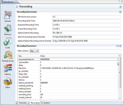
This tab contains meta information about the recording, such as its duration and the values of all the recording parameters used. This information can, among other things, be used to check if information is missing from a recording, or if that particular piece of information had simply been disabled for the recording.
The Memory tab group contains tabs that deal with memory-related information, such as heap usage and garbage collections. In JRA there are six such tabs, Overview, GCs, GC Statistics, Allocation, Heap Statistics, Heap Contents, and Object Statistics.
The first tab in the Memory tab group is the Overview tab. It shows an overview of the key memory statistics, such as the physical memory available on the hardware on which the JVM was running. It also shows the GC pause ratio, i.e. the time spent paused in GC in relation to the duration of the entire recording.
If the GC pause ratio is higher than 15-20%, it usually means that there is significant allocation pressure on the JVM.
At the bottom of the Overview tab, there is a listing of the different garbage collection strategy changes that have occurred during recording. See Chapter 3, Adaptive Memory Management, for more information on how these strategy changes can occur.
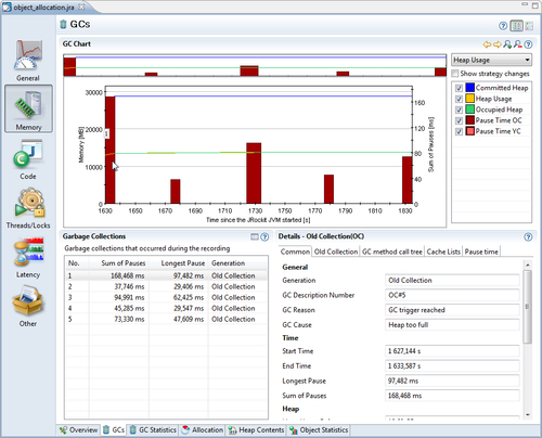
Here you can find all the information you would ever want to know about the garbage collections that occurred during the recording, and probably more.
With the GCs tab, it is usually a good idea to sort the Garbage Collections table on the attribute Longest Pause, unless you know exactly at what time from the start of the JVM you want to drill down. You might know this from reading the application log or from the information in some other tab in JRA. In the following example, the longest pause also happens to be the first one.
It is sometimes a good idea to leave out the first and last garbage collections from the analysis, depending on the recording settings. Some settings will force the first and last GC in the recording to be full garbage collections with exceptional compaction, to gather extra data. This may very well break the pausetime target for deterministic GC. This is also true for JRockit Flight Recorder
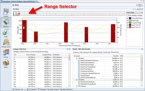
At the top of the screen is the Range Selector. The Range Selector is used to temporally select a set of events in the recording. In this case, we have zoomed in on a few of the events at the beginning of the recording. We can see that throughout this range, the size of the occupied heap (the lowest line, which shows up in green) is around half the committed heap size (the flat topmost line, which shows up in blue), with some small deviations.
In an application with a very high pause-to-run ratio, the occupied heap would have been close to the max heap. In that case, increasing the heap would probably be a good start to increase performance. There are various ways of increasing the heap size, but the easiest is simply setting a maximum heap size using the -Xmx flag on the command line. In the example, however, everything concerning the heap usage seems to be fine.
In the Details section, there are various tabs with detailed information about a selected garbage collection. A specific garbage collection can be examined more closely, either by clicking in the GC chart or by selecting it in the table.
Information about the reason for a particular GC, reference queue sizes, and heap usage information is included in the tabs in the Details section. Verbose heap information about the state before and after the recording, the stack trace for the allocation that caused the GC to happen, if available, and detailed information about every single pause part can also be found here.
In the previous screenshot, a very large portion of the GC pause is spent handling the reference queues. Switching to the References and Finalizers chart will reveal that the finalizer queue is the one with most objects in it.
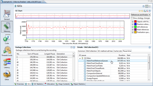
One way to improve the memory performance for this particular application would be to rely less heavily on finalizers. This is, as discussed in Chapter 3, always a good idea anyway.
Note
The recordings shown in the GCs tab examples earlier were created with JRockit R27.1, but are quite good examples anyway, as they are based on real-life data that was actually used to improve a product. As can be seen from the screenshot, there is no information about the start time of the individual pause parts. Recordings made using a more recent version of JRockit would contain such information. We are continuously improving the data set and adding new events to recordings. JRockit Flight Recorder, described in the next chapter, is the latest leap in recording detail.
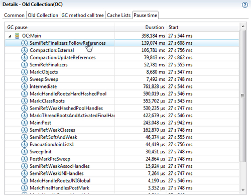
Following is a more recent recording with an obvious finalizer problem. The reasons that the pause parts differ from the previous examples is both that we are now using a different GC strategy as well as the fact that more recent recordings contain more detail. The finalizer problem stands out quite clearly in the next screenshot.
The data in the screenshot is from a different application, but it nicely illustrates how a large portion of the garbage collection pause is spent following references in the finalizers. Handling the finalizers is even taking more time than the notorious synchronized external compaction. Finalizers are an obvious bottleneck.
To make fewer GCs happen altogether, we need to find out what is actually causing the GCs to occur. This means that we have to identify the points in the program where the most object allocation takes place. One good place to start looking is the GC Call Trees table introduced in the next section. If more specific allocation-related information is required, go to the Object Allocation events in the Latency tab group.
For some applications, we can lower the garbage collection pause times by tuning the JRockit memory system. For more about JRockit tuning, see Chapter 5.
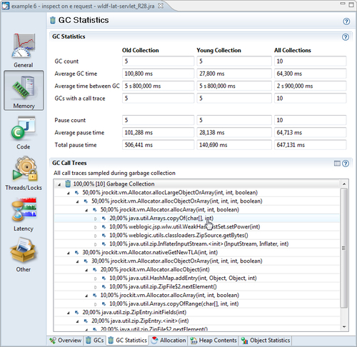
This tab contains some general statistics about the garbage collections that took place during the recording. One of the most interesting parts is the GC Call Trees table that shows an aggregated view of the stack traces for any garbage collection. Unfortunately, it shows JRockit-specific internal code frames as well, which means that you may have to dig down a few stack frames until the frames of interest are found—i.e., code you can affect.
Note
Prior to version R27.6 of JRockit, this was one of the better ways of getting an idea of where allocation pressure originated. In more recent versions, there is a much more powerful way of doing allocation profiling, which will be described in the Histogram section.
In the interest of conserving space, only the JRockit internal frames up to the first non-internal frame have been expanded in the following screenshot. The information should be interpreted as most of the GCs are being caused as the result of calls to Arrays.copyOf(char[], int) in the Java program.
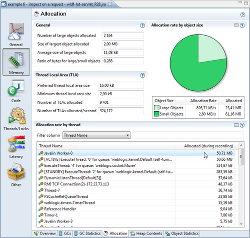
The Allocation tab contains information that can be used mainly for tuning the JRockit memory system. Here, relative allocation rates of large and small objects are displayed, which affects the choice of the Thread Local Area (TLA) size. TLAs are discussed to a great extent in Chapter 3 and Chapter 5. Allocation can also be viewed on a per-thread basis, which can help find out where to start tuning the Java program in order to make it stress the memory system less.
Again, a more powerful way of finding out where to start tuning the allocation behavior of a Java program is usually to work with the Latency | Histogram tab, described later in this chapter.
Information on the memory distribution of the heap can be found under the Heap Contents tab. The snapshot for this information is taken at the end of the recording. If you find that your heap is heavily fragmented, there are two choices—either try to tune JRockit to take better care of the fragmentation or try to change the allocation behavior of your Java application. As described in Chapter 3, the JVM combats fragmentation by doing compaction. In extreme cases, with large allocation pressure and high performance demands, you may have to change the allocation patterns of your application to get the performance you want.
The Object Statistics tab shows a histogram of what was on the heap at the beginning and at the end of the recording. Here you can find out what types (classes) of objects are using the most memory on the heap. If there is a large positive delta between the snapshots at the beginning and at the end of the recording, it means that there either is a memory leak or that the application was merely executing some large operation that required a lot of memory.
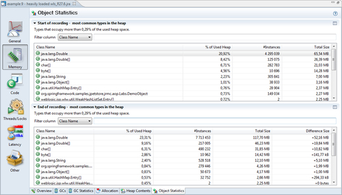
In the previous example, there is actually a memory leak that causes instances of Double to be held on to forever by the program. This will eventually cause an OutOfMemoryError.
The best way to find out where these instances are being created is to either check for Object Allocation events of Double (see the second example in the Histogram section) or to turn on allocation profiling in the Memory Leak Detector. The Memory Leak Detector is covered in detail in Chapter 10, The Memory Leak Detector.
The Code tab group contains information from the code generator and the method sampler. It consists of three tabs—the Overview, Hot Methods, and Optimizations tab.
This tab aggregates information from the code generator with sample information from the code optimizer. This allows us to see which methods the Java program spends the most time executing. Again, this information is available virtually "for free", as the code generation system needs it anyway.
For CPU-bound applications, this tab is a good place to start looking for opportunities to optimize your application code. By CPU-bound, we mean an application for which the CPU is the limiting factor; with a faster CPU, the application would have a higher throughput.
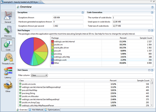
In the first section, the amount of exceptions thrown per second is shown. This number depends both on the hardware and on the application—faster hardware may execute an application more quickly, and consequently throw more exceptions. However, a higher value is always worse than a lower one on identical setups. Recall that exceptions are just that, rare corner cases. As we have explained, the JVM typically gambles that they aren't occurring too frequently. If an application throws hundreds of thousands exceptions per second, you should investigate why. Someone may be using exceptions for control flow, or there may be a configuration error. Either way, performance will suffer.
Note
In JRockit Mission Control 3.1, the recording will only provide information about how many exceptions were thrown. The only way to find out where the exceptions originated is unfortunately by changing the verbosity of the log, as described in Chapter 5 and Chapter 11. As the next chapter will show, exception profiling using JRockit Flight Recorder is both easier and more powerful.
An overview of where the JVM spends most of the time executing Java code can be found in the Hot Packages and Hot Classes sections. The only difference between them is the way the sample data from the JVM code optimizer is aggregated. In Hot Packages, hot executing code is sorted on a per-package basis and in Hot Classes on a per-class basis. For more fine-grained information, use the Hot Methods tab.
As shown in the example screenshot, most of the time is spent executing code in the weblogic.servlet.internal package. There is also a fair amount of exceptions being thrown.
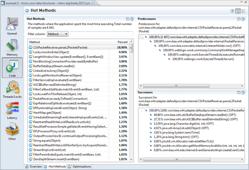
This tab provides a detailed view of the information provided by the JVM code optimizer. If the objective is to find a good candidate method for optimizing the application, this is the place to look. If a lot of the method samples are from one particular method, and a lot of the method traces through that method share the same origin, much can potentially be gained by either manually optimizing that method or by reducing the amount of calls along that call chain.
In the following example, much of the time is spent in the method com.bea.wlrt.adapter.defaultprovider.internal.CSVPacketReceiver.parseL2Packet(). It seems likely that the best way to improve the performance of this particular application would be to optimize a method internal to the application container (WebLogic Event Server) and not the code in the application itself, running inside the container. This illustrates both the power of the JRockit Mission Control tools and a dilemma that the resulting analysis may reveal—the answers provided sometimes require solutions beyond your immediate control.
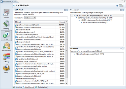
Sometimes, the information provided may cause us to reconsider the way we use data structures. In the next example, the program frequently checks if an object is in a java.util.LinkedList. This is a rather slow operation that is proportional to the size of the list (time complexity O(n)), as it potentially involves traversing the entire list, looking for the element. Changing to another data structure, such as a HashSet would most certainly speed up the check, making the time complexity constant (O(1)) on average, given that the hash function is good enough and the set large enough.
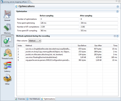
This tab shows various statistics from the JIT-compiler. The information in this tab is mostly of interest when hunting down optimization-related bugs in JRockit. It shows how much time was spent doing optimizations as well as how much time was spent JIT-compiling code at the beginning and at the end of the recording. For each method optimized during the recording, native code size before and after optimization is shown, as well as how long it took to optimize the particular method
The Thread/Locks tab group contains tabs that visualize thread- and lock-related data. There are five such tabs in JRA—the Overview, Thread, Java Locks, JVM Locks, and Thread Dumps tab.
The Overview tab shows fundamental thread and hardware-related information, such as the number of hardware threads available on the system and the number of context switches per second.
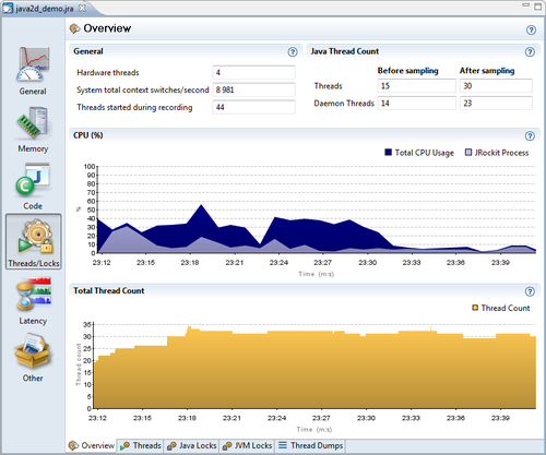
A dual-core CPU has two hardware threads, and a hyperthreaded core also counts as two hardware threads. That is, a dual-core CPU with hyperthreading will be displayed as having four hardware threads.
A high amount of context switches per second may not be a real problem, but better synchronization behavior may lead to better total throughput in the system.
There is a CPU graph showing both the total CPU load on the system, as well as the CPU load generated by the JVM. A saturated CPU is usually a good thing—you are fully utilizing the hardware on which you spent a lot of money! As previously mentioned, in some CPU-bound applications, for example batch jobs, it is normally a good thing for the system to be completely saturated during the run. However, for a standard server-side application it is probably more beneficial if the system is able to handle some extra load in addition to the expected one.
Note
The hardware provisioning problem is not simple, but normally server-side systems should have some spare computational power for when things get hairy. This is usually referred to as overprovisioning, and has traditionally just involved buying faster hardware. Virtualization has given us exciting new ways to handle the provisioning problem. Some of these are discussed in Chapter 13, JRockit Virtual Edition.
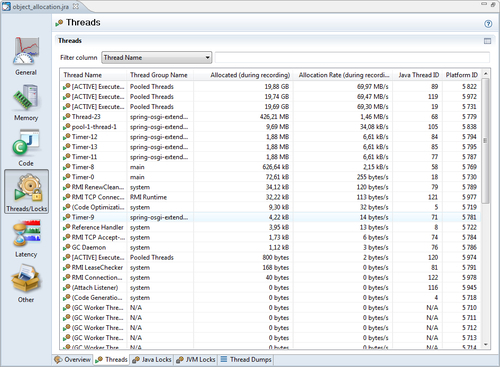
This tab shows a table where each row corresponds to a thread. The tab has more to offer than first meets the eye. By default, only the start time, the thread duration, and the Java thread ID are shown for each thread. More columns can be made visible by changing the table properties. This can be done either by clicking on the Table Settings icon, or by using the context menu in the table.
As can be seen in the example screenshot, information such as the thread group that the thread belongs to, allocation-related information, and the platform thread ID can also be displayed. The platform thread ID is the ID assigned to the thread by the operating system, in case we are working with native threads. This information can be useful if you are using operating system-specific tools together with JRA.
This tab displays information on how Java locks have been used during the recording. The information is aggregated per type (class) of monitor object. For more information regarding the different kind of locks, please refer to Chapter 4, Threads and Synchronization.
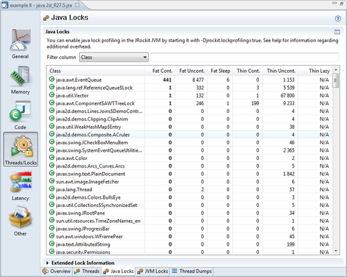
This tab is normally empty. You need to start JRockit with the system property jrockit.lockprofiling set to true, for the lock profiling information to be recorded. This is because lock profiling may cause anything from a small to a considerable overhead, especially if there is a lot of synchronization.
Note
With recent changes to the JRockit thread and locking model, it would be possible to dynamically enable lock profiling. This is unfortunately not the case yet, not even in JRockit Flight Recorder.
For R28, the system property jrockit.lockprofiling has been deprecated and replaced with the flag -XX:UseLockProfiling.
This tab contains information on JVM internal native locks. This is normally useful for the JRockit JVM developers and for JRockit support.
Note
Native locks were discussed to some extent in Chapter 4. An example of a native lock would be the code buffer lock that the JVM acquires in order to emit compiled methods into a native code buffer. This is done to ensure that no other code generation threads interfere with that particular code emission.
The latency tools were introduced as a companion to JRockit Real Time. The predictable garbage collection pause times offered by JRockit Real Time made necessary a tool to help developers hunt down latencies introduced by the Java application itself, as opposed to by the JVM. It is not enough to be able to guarantee that the GC does not halt execution for more than a millisecond if the application itself blocks for hundreds of milliseconds when, for example, waiting for I/O.
When working with the tabs in the Latency tab group, we strongly recommend switching to the Latency perspective. The switch can be made from the menu Window | Show Perspective. In the latency perspective, two new views are available to the left—the Event Types view and the Properties view. The Event Types view can be used to select which latency events to examine and the Properties view shows detailed information on any selected event.
Similar to in the GCs tab, at the top of all the latency tabs is the Range Selector. The range selector allows you to temporarily select a subset of the events and only examine this subset. Any changes either to the Event Types view or the range selector will be instantly reflected in the tab. The graph in the backdrop of the range selector, normally colored red, is the normalized amount of events at a specific point in time. The range selector also shows the CPU load as a black graph rendered over the event bars. It is possible to configure what should be displayed using the range selector context menu.
The operative set is an important concept to understand when examining latencies and subsets of latencies. It is a set of events that can be added to and removed from, by using the different tabs in the latency tab group. Think of it as a collection of events that can be brought from one tab to another and which can be modified using the different views in the different tabs. Understanding and using the operative set is very important to get the most out of the latency analysis tool.
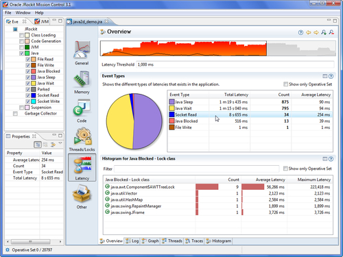
The Overview tab provides an aggregated view of the latency events in the recording. At the top, just under the range selector, the Latency Threshold used during the recording can be seen. As potentially very large volumes of data can be recorded, the Latency Threshold is normally used to limit the amount of events so that only the ones longer than a certain threshold are actually recorded. The default is to only record latency events that are longer than 20 milliseconds.
Note
A latency event is any time slice longer than a preset value that the JVM spends not executing Java code. For example, it may instead be waiting for data on a socket or performing a phase of garbage collection that stops the world.
The Event Types histogram and accompanying pie chart show breakdowns per event type. This is useful to quickly get a feel for what kind of events were recorded and their proportions. Note that the pie chart shows the number of events logged, not the total time that the events took. A tip for finding out where certain types of events are occurring is to use the context menu in the Event Types histogram to add the events of a certain type to the operative set. This causes the events of that type to be colored turquoise in the range selector.
Another tip is to go to the Traces view and click on Show only Operative Set, to see the stack traces that led up to the events of that particular type.
The latency Log tab shows all the available events in a table. The table can be used for filtering events, for sorting them, and for showing the events currently in the operative set. It is mostly used to quickly sort the events on duration to find the longest ones. Sometimes, the longest latencies may be due to socket accepts or other blocking calls that would actually be expected to take a long time. In such cases, this table can be used to quickly find and remove such events from the operative set, concentrating only on the problematic latencies.
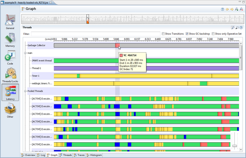
The latency Graph tab contains a graph where the events are displayed, aggregated per thread. In the following example, we only show the events from the Java and Garbage Collector event types. The normal rendering procedure for the graph is that each event producer gets its own per-thread lane where the events for that particular producer are displayed. For each thread, only one event can occur in a lane at any given time. Garbage collection events are drawn in a slightly different way—they are always shown at the top of the latency event graph, and each GC is highlighted as a backdrop across all the other threads. This is useful for seeing if a certain latency event was caused by a garbage collection. If part of a lane in the latency graph is green, it means that the thread is happily executing Java code. Any other color means that a latency event is taking place at that point in time. To find out what the color means, either hover the mouse over an event and read the tooltip, or check the colors in the Event Types view.
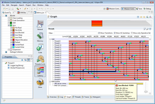
The latency Graph can also show thread transitions. The application in the next screenshot has an exaggerated pathological behavior, where all threads in an application are sharing a logger through a static field, and where the logger is using a synchronized resource for writing log data. As can be seen, the worker threads are all waiting on the shared resource. The worker threads that are there to execute parts of the work in parallel, rely on the shared logger. This actually causes the entire application to execute the work in a sequential fashion instead.
If you see an event that you want to get more information on, you can either select it in the graph and study it in the properties view, hover the mouse pointer over it and read the tooltip that pops up, or add it to the operative set for closer examination in one of the other views.
To summarize, the Graph view is good for providing an overview of the latency and thread behavior of the application.
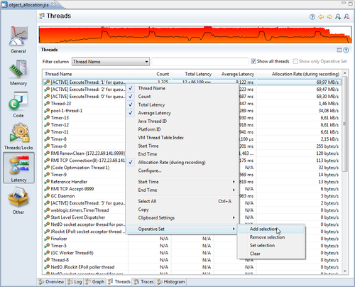
The Threads tab is basically a table containing the threads in the system, much like the threads tab in the Management Console, as described in Chapter 7. The most useful properties in this table tend to be the event Count and the Allocation Rate per thread.
This view is mainly used to select a specific thread, either based on an attribute, such as the one with the highest allocation rate, or for finding a specific thread by name. The operative set is then used to select the events for that particular thread, so that the events can be studied in the other views. Sets of threads can also be selected.
This is where the stack traces for sets of events get aggregated. For instance, if the operative set contains the set of allocation events for String arrays, this is the tab you would go to for finding out where those object allocations take place. In the next example, only the traces for the operative set are visible. As can be seen, the Count and Total Latency columns have bar chart backdrops that show how much of the max value, relative to the other children on the same level, the value in the cell corresponds to. Everything is normalized with respect to the max value.
Normally, while analyzing a recording, you end up in this tab once you have used the other tabs to filter out the set of events that you are interested in. This tab reveals where in the code the events are originating from.
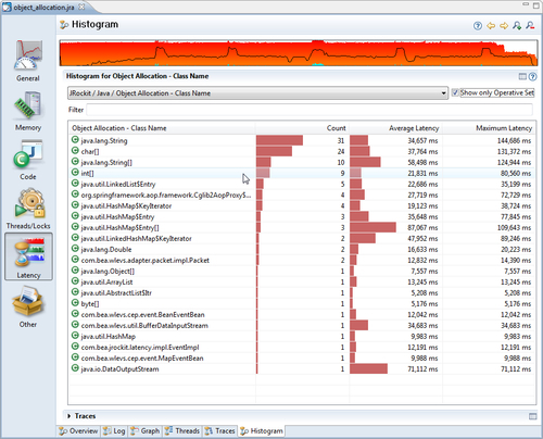
This very powerful tab is used to build histograms of the events. The histogram can be built around any event value. A few examples of useful ones are:
- Object Allocation | Class Name: For finding out what types of allocations are most common
- Java Blocked | Lock Class: For finding out which locks are most frequently blocking in the application
- Java Wait | Lock Class: For finding out where the application spends the most time in
wait()
Once the interesting events have been found, they are usually added to the operative set and brought to another tab for further investigation.
Sadly, one of the most overlooked features in JRA is the operative set. This example will explain how the operative set can be used to filter out a very specific set of events to solve a specific problem. In this example, we have been given a JRA recording from another team. The team is unhappy with the garbage collections that take place in an application. Garbage collections seem to be performed too frequently and take too long to complete. We start by looking at the GCs tab in the Memory section.
The initial reaction from examining the garbage collections is that they are indeed quite long, tens of milliseconds, but they do not happen all that often. For the duration of the recording only five GCs took place. We could probably ask the clients to switch to deterministic GC. This would cause more frequent but much shorter garbage collections. However, as we are curious, we would like to get back to them with more than just a GC strategy recommendation. We would still like to know where most of the pressure on the memory system is being created.
As this is an example, we'll make this slightly more complicated than necessary, just to hint at the power of JRA. We switch to the latency data thread tab and look for the most allocation intensive threads. Then we add these events to the Operative Set. It seems that almost all allocation is done in the top three threads.
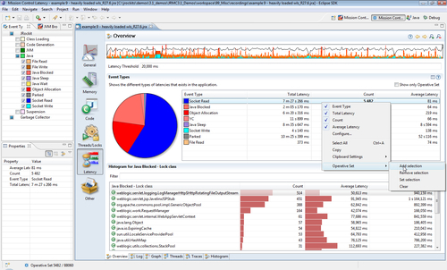
We have now added all the events for the three threads to our Operative Set, but we are only interested in studying the allocation behavior. In order to do this, we move to the Histogram tab and build a histogram for the allocation events in our Operative Set.
Note that object allocations are weird latency events, as we are normally not interested in their duration, but rather the number of occurrences. We therefore sort them on event count and see that most of the object allocation events in our three threads are caused by instantiating Strings. As we're eager to find out where these events take place, we limit the operative set to the String allocation events.
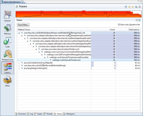
We proceed to the Traces view with our trimmed Operative Set, and once again check the Show only Operative Set button.
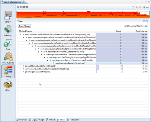
We quickly see that almost all the String instances in our three most allocation-intensive threads are allocated by the same method —readPaddedASCIIString(char [], int). If we also add char arrays, we can see that the char arrays are mostly created as a result of allocating the String objects in the same method. This makes sense as each String wraps one char array.
We can now recommend the team not only to change GC strategies, but we can also say for sure, that one way to drastically reduce the pressure on the memory system in this particular application would be to either create less strings in the method at the top in the Traces view, or to reduce the number of calls along the path to that method.