1.4 LAGRANGE MULTIPLIER METHOD – AN OVERVIEW

Nonlinear function optimization problems such as ED can be solved by the Lagrange multiplier method.

1.4.1 Nonlinear Function Optimization Considering Equality Constraints

Let the problem be to minimize the function

Subject to k number of equality constraints

The constrained function f can be written as an unconstrained function with the help of the Lagrange method as:

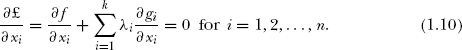
In Eq. (1.12) £ is the Lagrange function and λ is the Lagrange multiplier. The necessary condition for minimum £ can be obtained from:

= g_i = 0 for i = 1, 2, … , k.                    (1.11)

Equations (1.11) represents the original constraints. This method is adopted to solve the ED problem and is explained in detail in the following sections.

Example 1.2

Minimize

Subject to g (x, y) = x² + y² – 64 = 0

Solution:

The Lagrange function is:

The necessary conditions for the minimization of f (x, y) is given by

From (1),

From (2),

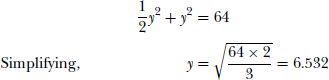
From (4) and (5), the relation can be obtained.

This relation, along with (3), gives the optimum solution.

Replacing y in (3),

                                        x² + 2x² = 64

(or)                                          3x² = 64

and                                              x = 4.618

replacing x in (3),

1.4.2 Nonlinear Function Optimization Considering Equality and Inequality Constraints

Majority of optimization problems contain both equality and inequality constraints. Let the problem be to minimize the function:

subject to k number of equality constraints

and m number of inequality constraints

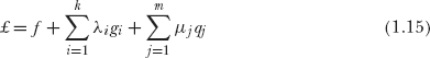
The inequality constraints, as mentioned earlier, are independent control parameters or undetermined quantities. These constraints are bounded to certain limits. By introducing m vector of μ undetermined quantities, the constrained function f can be written as an unconstrained function with the help of Lagrange method as:

The necessary condition for minimum ₤ can be obtained from:

Note that Eq.(1.17) is the original equality constraint. The necessary conditions discussed above are known as the Kuhn-Tucker conditions.

Example 1.3

Minimize f(x,y) = x² + y²

Subject to inequality constraint:

Subject to equality constraint:

Solution:

The constrained objective function can be converted into an unconstrained function by using the Lagrange method as:

The necessary conditions are:

Solving the above equations for x, y shall yield an optimal solution, which minimizes the objective function. The procedure is similar to that given in Example 1.2.