1.5 ECONOMIC DISPATCH PROBLEM – NEGLECTING TRANSMISSION LINE LOSSES
The problem of ED can be easily solved when transmission line losses are neglected. As the losses are neglected, the system model can be understood as shown in Fig. 1.7, where n number of generating units are connected to a common bus bar, collectively meeting the total power demand PD. It should be understood that share of power demand by the units does not involve losses.
Since transmission losses are neglected, total demand PD is the sum of all generations of n-number of units. For each unit, a cost functions Ci is assumed and the sum of all costs computed from these cost functions gives the total cost of production CT.
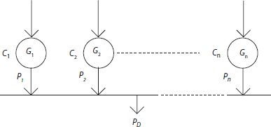
Fig 1.7 System with n-generators
where the cost function of the ith unit, from Eq. (1.1) is:
Now, the ED problem is to minimize CT, subject to the satisfaction of the following equality and inequality constraints.
Equality constraint
The total power generation by all the generating units must be equal to the power demand.
where Pi = power generated by ith unit
PD = total power demand.
Inequality constraint
Each generator should generate power within the limits imposed.
Economic dispatch problem can be carried out by excluding or including generator power limits, i.e., the inequality constraint.
1.5.1 Solution of Economic Dispatch Problem – Neglecting Losses and Generator Limits
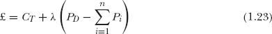
The constrained total cost function Eq. (1.20) can be converted into an unconstrained function by using the Lagrange multiplier as:
The conditions for minimization of objective function can be found by equating partial differentials of the unconstrained function to zero as
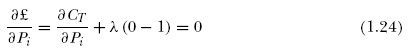
From Eq. (1.24)
Since Ci = C1 + C2+…+Cn
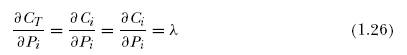
From the above equation the coordinate equations can be written as:
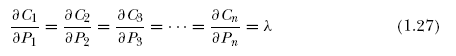
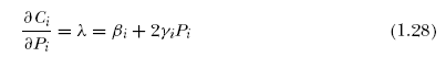
Using Eq. (1.2),
The second condition can be obtained from the following equation:
Equations Required for the ED solution
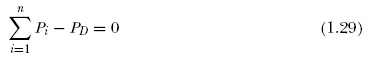
For a known value of λ, the power generated by the ith unit from Eq. (1.29) can be written as:
Eq. (1.30) is valid, subject to the satisfaction of the equality constraint, which can be written as:
From Eq. (1.31) the required value of λ is:
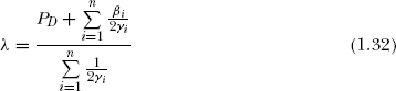
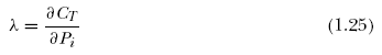
The value of λ can be calculated from Eq. (1.32) and then can be substituted in Eq. (1.31) to compute the values of Pi for i = 1, 2,…, n for optimal scheduling of generation.
1.5.2 Algorithm – Economic Dispatch Without Considering Generator Limits
Step 1: Read data: Cost coefficients αi,βi, γi, and total power demand PD.
Step 2: Compute λ value by using Eq. (1.32).
Step 3: Obtain economic dispatch solution using the Eq. (1.31) for all the units.
The incremental costs of the two generating units are as follows:
Given that the minimum and maximum powers are 10MW and 100MW for each unit, allocate a total load of 100 MW optimally.
Solution:
The incremental production cost of the two generating units is given as
For optimal scheduling equate (1) and (2)
Simplifying the above,
Given total load = 100 MW
Hence P1 + P2 = 100MW
Solving equations (3) and (4) we get
Both units are operating within their generation limits.
Example 1.5
For the two units in Example 1.4, instead of allocating load optimally, the load is shared equally. Calculate the net loss in Rs/hr for the process.
Solution:
If loads are shared equally, then the load supplied to the units will be 50 MW each
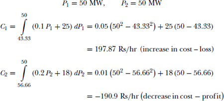
Table 1.4
|
Time |
Total load |
|
12 Midnight–6 AM |
50 MW |
|
6 AM–12 Noon |
120 MW |
|
12 Noon–3 PM |
180 MW |
|
3 PM–10 PM |
200 MW |
|
10 PM–12 Midnight |
80 MW |
So. if load is shared equally,
Net cost = C1 + C2 = (197.87) + (–190.9) = 6.97 Rs/hr. (net loss)
Example 1.6
The load for the power system consisting of two units in Example 1.3 is varied as shown in Table 1.4. For the shown load variations, allocate the load optimally.
Solution:
The incremental costs of the two units are
For optimal scheduling equate (1) and (2).
- When total load is 50 MW (12 Midnight – 6 A.M)
P1 + P2 = 50 (4)
Solving equations (3) and (4)
P1 = 10 MW P2 = 40 MW - When total load is 120 MW (6 A.M – 12 Noon)
P1 + P2 = 120 (5)
Solving equations (3) and (5)
P1 = 56.66 MW P2 = 63.33 MW - When total load is 180 MW (12 Noon – 3 P.M)
P1 + P2 = 180 (6)
Solving equations (3) and (6)
P1 = 96.66 MW P2 = 83.33 MW - When total load is 200 MW (3 P.M – 10 P.M)
P1 + P2 = 200 (7)
Solving equations (3) and (7)
P1 = 110 MW P2 = 90 MW - When total load is 80 MW (10 P.M – 12 Midnight)
P1 + P2 = 80 (8)
Solving equations (3) and (8)
P1 = 30 MW P2 = 50 MW
Example 1.7
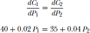
Incremental fuel cost of two generating units are: IC1 = 30 + 0.2 P1; IC2 = 25 + 0.3 P2 Rs/MWh, respectively. Find the savings in fuel cost in rupees annually for optimal scheduling of a total load of 140 MW, as compared to equal distribution of the same load between the two units.
Solution:
Incremental fuel cost of two generators are given as
For optimal scheduling IC1 = IC2
For equal sharing of load P1 = P2 = 70MW
For saving in fuel cost
Integrating the above equation within the limits, we calculate the change in fuel cost ΔF1
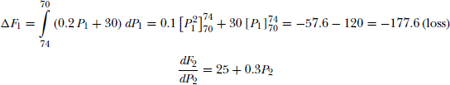
Integrating the above equation within the limits we calculate ΔF2
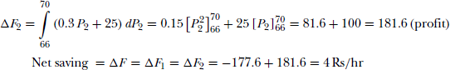
Net saving in rupees annually = 4 Rs/hr × 8760 hrs in a year = Rs 35,040/-
Example 1.8
The fuel cost functions for three thermal units in Rs/hr are given by:
where P1, P2 and P3 are in MW. For a total load of 1000 MW, find the economic dispatch solution.
Solution:
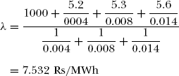
Using Eq. (1.33), λ is found to be
Substituting for λ in Eq. (1.31), the optimal dispatch is:
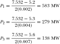
Equality constraint ![]()
i.e., 1000 – (583 + 279 + 138) = 0 is satisfied.
1.5.3 Solution of Economic Dispatch Problem – Neglecting Losses and Including Generator Limits
For the satisfactory operation of a thermal unit, the power generated by it should not be more than Pmax or less than Pmin This constraint needs to be satisfied owing to thermal lismits imposed on the unit. Now the problem of economic dispatch is, the minimization of the total cost of generation subject to the equality constraint given by Eq. (1.21) and the inequality constraint given by Eq. (1.22).
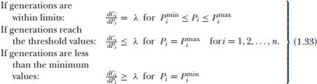
Following the discussion in Section 1.4.2, the necessary Kuhn–Tucker conditions that minimize the Lagrange function by including inequality constraints given by Eq(1.22) are:
Numerical Solution
Estimate the value of λ using Eq. (1.32). Compute the corresponding Pi values using Eq. (1.30). Then the equality constraint ![]() is verified subject to the satisfaction of inequality constraints, i.e., generation limits. If satisfied, λ value is taken to determine optimal power generation. Otherwise, λ value must be modified as per the gradient method described in this section. Rewrite Eq. (1.32) as:
is verified subject to the satisfaction of inequality constraints, i.e., generation limits. If satisfied, λ value is taken to determine optimal power generation. Otherwise, λ value must be modified as per the gradient method described in this section. Rewrite Eq. (1.32) as:
Expand the left-hand side of Eq. (1.34) using the Taylor’s series approximation and neglect higher order terms. Using the rth iteration value of λ,
Let ΔP(r) = PD − f (λ)(r)
Eq. (1.35) can be written as:
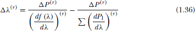
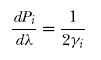
From Eq (1.30)
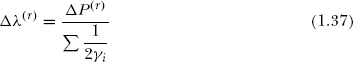
Hence the modified value of λ for the (r + 1)th iteration is:
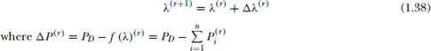
As the value of λ is modified, the Σ Pi reaches PD. If any Pi exceeds the maximum or goes below the minimum values, then P1 is set to that corresponding limit and maintained constant thereafter. After Pi is maintained constant, for optimal allocation of load, only the other units that have not violated the limits must be considered. In other words, all the units other than i must operate at equal incremental costs. This procedure is continued till ΣPi equals PD.
1.5.4 Algorithm – Economic Dispatch Including Generator Power Limits
|
Step 1: |
Read data: Cost coefficients of all n-units αi, βi, γi, for i = 1, 2,…, n; total power demand PD, convergence tolerance value |
|
Step 2: |
Obtain λ value using Eq. (1.32). or assume a suitable λ value. |
|
Step 3: |
Allocate PD optimally and obtain the values of Pi (i = 1, 2, …, n) by using Eq. (1.30). |
|
Step 4: |
Check condition: each Pi for Pi(min) ≤ Pi ≤ Pi(max) (i = 1, 2,…, n) |
|
|
Check condition: |
|
Step 6: |
Set iteration count, r = 1 |
|
Step 7: |
for i = 1, 2, …,n |
|
Compute |
|
|
Step 9: |
Compute Δλ(r) using Eq. (1.37). |
|
Step 10: |
Compute λ(r+1) using Eq. (1.38). |
|
Step 11: |
Allocate PD optimally among all the units other than i. Obtain the values of Pk(K = 1, 2, …, n) but k is not equal to i) by using Eq. (1.31). All the units and non-violating limits must operate at equal incremental costs. |
|
Step 12: |
Check the limits of generators: |
|
Step 13: |
Compute the optimal total cost using Eqs. (1.7) and (1.20) |
Example 1.9
The fuel cost of two generating units are as follows:
The generating limits are:
For a total load of 750 MW, find the optimal dispatch solution:
- without considering generator limits,
- considering generator limits.
Solution:
Fuel costs of the two generating units
Total load = 750 MW
- Optimal scheduling without considering generator limits:
Simplifying the above, 0.02 P1 − 0.04 P2 = −5 (3)
Further, P1 + P2 = 7500 (4)
solving (3) and (4) we get P1 = 416.66 MW P2 = 333.33 MW
- Considering generator limits:
Since P1 exceeds the upper limit.
Set P2 = 250 MW constantly.
Hence P2 = 750 – 250 = 500 MW.
Example 1.10
Three generating units have a total capacity of 500 MW. The incremental costs of production are given as follows:
Allocate a total load of 100 MW optimally amongst the three units.
Solution:
The incremental costs of production of the three units are:
For optimal scheduling λ = IC1 = IC2 = IC3
The approximate value of λ can be estimated by using Eq. (1.33). λ = 32.83 Using Eq. (1.31), the generation of each unit is computed as
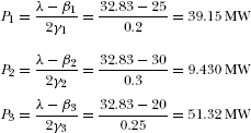
For the estimated λ, P1 and P3 are within the specified limits. But P2 violates the lower limit.
Therefore, set P2 to its lower limit, i.e., P2 = 30 MW.
P1(1) = 39.15 MW, P2 = 30 MW and P3(1) = 51.32 MW for λ(1) = 32.83
ΔP(1) = (100) − (39.15 + 30 + 51.32) = −20.47 MW
Using Eq. (1.39) the increment in λ can be computed as:
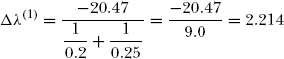
Now, the new value of λ is
Repeat the above for the next iteration.
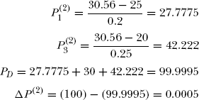
Since ΔP2 ≅ 0, we can stop the iteration process.
Since P1 and P2 are within the limits and the given equality constraints are satisfied, optimal allocation is
Example 1.11
Two units of 220 MW in a thermal plant are operating with a minimum load of 50 MW each, are having incremental cost of production as follows:
If the total load varies between 100 to 440 MW, obtain an optimal scheduling of the total load between the units.
Solution:
Incremental cost of production of the two units are:
The total load varies from 100Mw to 440 MW.
Let the total load = 100 MW.
As the minimum load on each unit is 50 MW, optimal allocation is not possible at this load.
Hence, generations to minimum P1 = 50 P2 = 50.
The λ value at minimum load is:
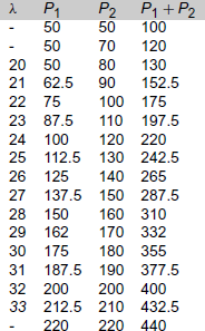
As seen above, Unit 1 operates at a higher incremental fuel cost than Unit 2. Therefore, any additional load above 50 MW can be allocated to Unit 2 till λ value of both units are equal.
Between 100 and 130 MW. The value of P1 is constant at 50 MW and P2 varies from 50 to 80 MW. Optimum allocation of load begins when total load value is at least 130 MW. Allocation of load between the two units for different values of λ is given in Table 1.5.
Again, optimum allocation of the total load of 440 MW is not possible due to maximum generation constraints. For 440 MW, P1 = 220 MW and P2 = 220MW. At this load the two units work at different λ values.