2.4 SOLUTION OF THE ECONOMIC SCHEDULING PROBLEM – CONSIDERING TRANSMISSION LINE LOSSES

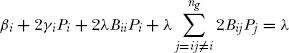
For optimal power dispatch, the incremental fuel cost of each plant multiplied by its penalty factor should be equal to Lagrangian multiplier λ.

 

where 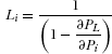= pentaly factor of i^th unit.

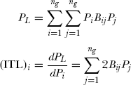
The incremental transmission loss can be obtained by differentiating the total loss equation P_L. The equation for P_L interms of B-coefficients has been developed earlier.

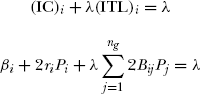
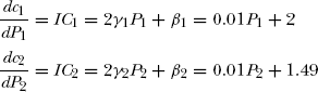
Recall the incremental cost of the i^th unit.

The incremental transmission loss(ITL) of the i^th unit is:

Substituting in the co-ordinate equation

 

 

or

Separating the i^th term,

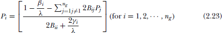
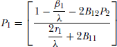
from the above, P_i is,

or

2.4.1 Algorithm

The algorithm for economic scheduling of plant load amongst n_g generating units involves the following steps:

1. Read generator characteristics i.e., β_i and r_i for i = 1, 2, …, n_g.
2. Read total plant load P_D and B-coefficients.
3. Choose initial value of λ = λ₀.
4. Set all P_i = 0, for i = 1, 2, …, n_g.
5. Set iteration count r = 1
6. Solve P_i^(r) from Eq.(2.24)
   

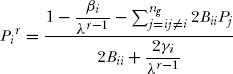
   for i = 1, 2, 3 …, n_g units

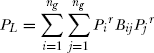
7. Using P_i values, compute P_L from
   
8. Check if equality constraint
   

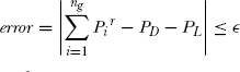
   (specified error) is satisfied or not.

   If YES, stop iteration process, print results. If NO, Goto Step-9.

9. If error value in step-8 is negative then increase λ and Δλ (a suitable increment) or, decrease λ by Δλ if error is positvie.
10. Repeat the iteration processly set r = r + 1; Goto Step-5.

P_i^min ≤ P_i^r ≤ P_i^max is not satisfied at the end of Step-6, then we set P_i = P_i^max or P_i^min to constant and scheduling is done only for the rest of the generating units.

The iterative procedure is illustrated with the following numerical examples.

Example 2.5

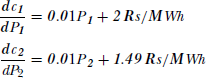
The incremental cost of production of two generating units are given as:

The B-coefficients in MW^-1 are given by

 

For a given cost of received power λ=2.5 Rs/MWh, compute economic power generation by the units, total losses in the system and total plant load.

Solution:

From the above,

 

Using Eq.(2.23),

Substituting numerical values

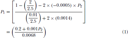
Again using Eq. (2.24)

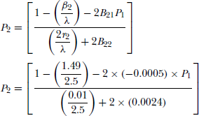
or

First iteration:

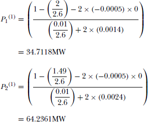
set P₁⁽⁰⁾ = P₂⁽⁰⁾ = 0 MW

Using (1)

Using (2)

Second iteration:

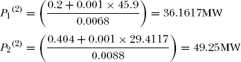
Third iteration:

 

 

Continuing the iteration process,

 

 

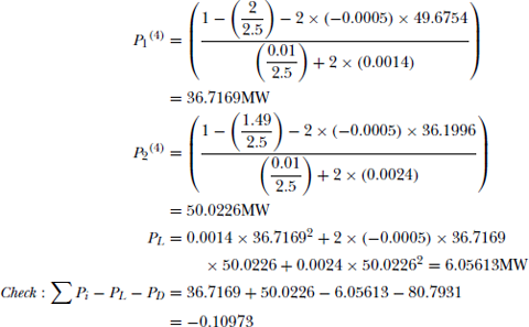
With accuracy up to the 4^th decimal, the optimal scheduling for λ = 2.5 Rs/MWh is:

 

 

Total loss at this generation is

 

            P_L = (0.0014 × 36.7776² + 2 × (−0.0005) × 36.7776 × 50.0883 + 0.0024 × 50.0883²)

                = 1.8936 − 1.8421 + 6.0212

                = 6.0727MW

 

Total load demand at this scheduling is:

or

Example 2.6

With loss coefficients and incremental production costs given in Example 2.5, allocate a total load of 80.7931 MW between the two units optimally and also determine the incremental cost of received power in Rs/MWh.

Solution:

 

Let λ° = 2.6;^† P₁° = P₂° = 0MW.

First iteration:

Using Eq.(2.24)

Transmission loss for the above generation is:

 

                P_L = 0.0014 × 34.7118² × 2 × (−0.0005) × 34.7118 × 64.2361 + 0.0024 × 64.2361²

                    = 9.3601MW

 

Check equality constraint.

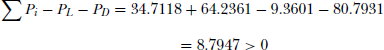
Since ∑ P_i – P_L – P_D > 0, λ value must decrease.

Second iteration:

Let λ⁽¹⁾ = 2.4

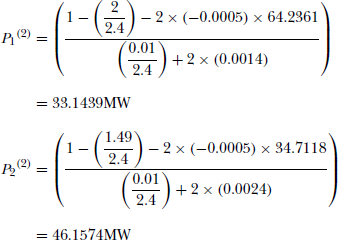
P₂ = 0.0014 × 33.1439² + 2 × (−0.0005) × 33.1439 × 46.1574 + 0.0024 × 46.1574²

= 5.1213MW

Check equality constraint.

Since ∑ P_i – P_L – P_D < 0, λ value should increase.

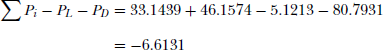
Third iteration:

Let λ⁽²⁾ = 2.5

Check equality constraint.

Since the error is small, λ can be fixed at 2.5Rs/MWh.

Next iteration:

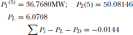
Final result:

 

                P₁ = 36.768MW;    P₂ = 50.08146MW

                P₂ = 6.0708MW;    Cost of received power = 2.5Rs/MWh

Example 2.7

The incremental fuel cost of two plants are:

 

 

The loss coefficients are given in the following matrix:

For the value of incremental cost of received power λ =Rs 25/MWh, find the economically scheduled generation of both plants, total load and losses.

Solution:

 

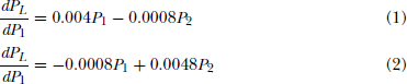
The total loss formula in B-coefficients is:

 

 

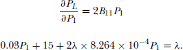
Differentiating P_L with respect to P₁ and P₂ gives the ITL of the two units

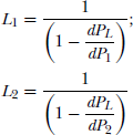
For optional scheduling,

 

where

From (3),

and

From (4)

Simplifying the above,

 

From (5),

Simplifying the above,

 

Solving (6) and (7),

 

 

Now the transmission loss at this generation is

 

                P₂ = 0.002 × 50² − 0.0008 × 50 × 75 + 0.0024 × 75²

                = 15.5MW

 

The total plant load is:

Example 2.8

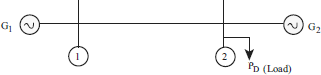
Consider a 2-Bus, two generator power system shown in the Fig. 2.6.

When 110MW power is transmitted from Bus-1 to load at Bus-2, a transmission loss of 10MW is incurred. The incremental fuel costs of G₁ and G₂ are:

 

 

Find the power received by the load and the optimal generation by G₁ and G₂ when the incremental cost of received power of the system is Rs 20/MWh

Solution:

 

As the total load is placed at Bus-2, B₂₂ = B₁₂ = B₂₁ = 0 (refer Example. 2.4)

The loss equation is:

 

 

For P₁ = 110MW; P₂ = 10MW (given).

Therefore,

For optimal scheduling,

 

 

or

or

where,

Substituting λ = 20,

 

 

From the above,

 

 

and

 

 

For optimal scheduling,

 

Therefore,

 

 

From the above,

Thus,

 

 

Therefore, P_D = Total load = ∑ P₁ – P₂ =174.105 MW

Example 2.9

The incremental cost of generation of two generating units are given as:

 

 

The optimal allocation of total plant load yields the generation of two units as P₁ = P₂ = 100MW. If the penalty factor of Unit-1 is 1.2, find the penalty factor of Unit-2

Solution:

 

Incremental cost of generation (IC) of two units at

P₁ = P₂ = 100MW is:

 

 

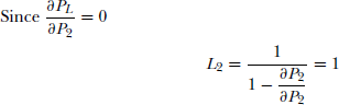
Considering losses, at optimal allocation the coordinate equation is:

 

 

i.e 40 × 1.2 = 30 × L₂

Therefore, L₂ = 1.6 (Penalty factor of Unit-2)