2.5 ECONOMIC DISPATCH CONSIDERING LOSSES – THE CLASSICAL METHOD

For fast and effective solution of the economic dispatch problem the following method which uses the gradients is proposed.

Recall the Eqn.(2.23) of r^th iteration as:

for i = 1, 2, …, n_g

We have the equality constraint

The r^th iteration values of P_i obtained from Eq.(2.23) are substituted in the above equality constraint equation.

That is,

where P^r_L is the total loss of the system computed using P_i, for i=1, 2,…, n_g. Eq.(2.25) takes the form:

Expanding Eq.(2.26) by Taylor’s series and neglecting higher order terms,

or

Where ΔP^r is the error in power balance computed from the equality constraint equation.

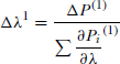
From Eq.(2.28), the increment in λ for the next iteration, Δλ^r is

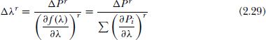
where

Note: Eq.(2.30) is obtained from the following formula:

Therefore, the r^th iteration value of λ is:

 

The iteration process is continued until ΔP^r is less than a specified error.

2.5.1 Algorithm

The algorithm for the economic dispatch problem involves the following steps.

Step-1: Read Data – α_i, β_i, γ_i for i=1, 2,…, n_g number of generators, B-coefficients, error specified ∈ and total plant road P_D.

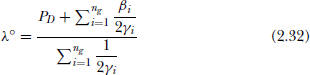
Step-2: Compute initial value of λ by using Eq.(2.32)

Step-3: Compute initial values of P_Gi for i=1, 2,…, n_g using Eq.(2.31)

Step-4: Set iteration count r = 1

Step-5: Compute P_i^r for i=1, 2,…, n_g by using P_i^r–1 and λ^r–1 values in Eq.(2.24).

Step-6: Compute transmission loss P_L^r using B-coefficients and generations (P_gi values) obtained in Step-5.

Step-7: Compute the error in power balance equation i.e ΔP^r from

Step-8: Check |ΔP^r| ≤ ∈

          IF ‘Yes’ GOTO Step-13

          ELSE GOTO Step-9

Step-9: Compute Δλ^r using Eq.(2.29).

Step-10: Update the value of λ as:

 

 

Step-11: Set r = r + 1

Step-12: GOTO Step-5

Step-13: Print Results, END

Example 2.10

The incremental cost of production of two generating units are given as:

 

 

The loss formula is given as:

 

 

where P₁ and P₂ are the generations of the two units. Using the gradient method, compute economic power generation by the units and total losses in the system. Assume plant load as 80.7931 MW.

Solution:

 

    We have

    2_γ1 = 0.01; 2_γ2 = 0.01; β₁ = 2; β₂ = 1.49;

    B₁₁ = 0.0014; B₁₂ = −0.0005; B₂₂ = 0.0024 from above,

 

Using Eq.(2.32), the initial value of λ is:

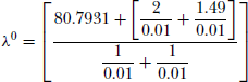
Solving,

 

 

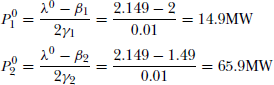
Initial values of generations P₁ and P₂ can be obtained by using Eq.(2.33) as:

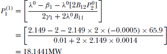
First Iteration:

The updated values of generations P₁ and P₂ can be obtained by using Eq.(2.24) as:

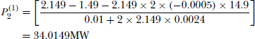
Similarly,

The transmission loss at these generations is:

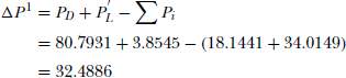
The error in power balance equation is:

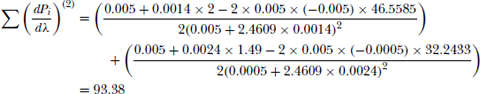
Now, the increment required for λ is:

Using Eq. (2.30)

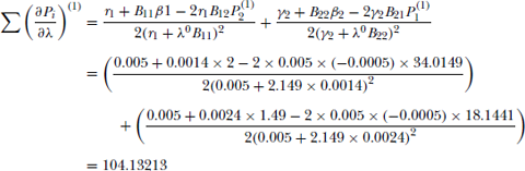
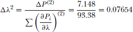
Now the increment for λ is:

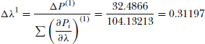
The updated value of λ is:

 

Second, Iteration

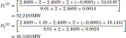
The initial values of P₁ and P₂ with updated value of λ are:

 

 

Using Eq. (2.24)

The transmission losses are:

 

P_L⁽²⁾ = 0.0014 × 32.2433² + 2 × (−0.0005) × 32.2433 × 46.5585 + 0.0024 × 46.5585²

    = 5.1567MW

ΔP⁽²⁾ = 80.7931 + 5.1567 − 32.2433 − 46.5585

    = 7.148MW

 

 

The increment for λ is:

The updated value of λ for the next increment is:

 

 

Note:

The student is advised to carry out a few more iterations and compare the results with results of Example 2.5

Example 2.11

In a 3-plant system the fuel cost functions of the generators are given by;

 

 

The loss equation in terms of B-coefficients is:

 

 

Find the economic dispatch for a total plant load of 750 MW

Solution:

 

The fuel cost equation is in the form:

 

 

Comparing the fuel cost equations of three generators

 

 

and

 

 

also, P_D = 750MW (given)

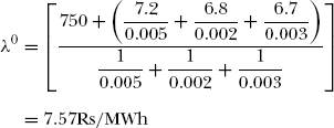
Using Eq. (2.32), the initial value of λ is:

First iteration:

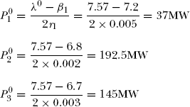
Initial values of generations P₁, P₂ and P₃ can be obtained by using Eq. (2.33) as:

The power loss at these generations is

 

                P_L = 0.0001 × 37² + 0.00002 × 192.5² + 0.00006 × 145²

                    = 2.139525MW

 

The error in the energy balance equality constraint is:

 

 

Using Eq (2.30),

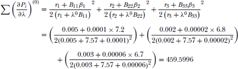
Now, the increment required for λ is:

The updated value of λ is:

 

                    λ⁽¹⁾ = λ⁰ + Δλ⁰ = 7.57 + 0.82167

                          = 8.39167Rs/MWH

 

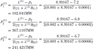
Second, iteration:

With the updated value of λ, the new generations can be obtained by using Eq.(2.24) as:

Loss at these generations is:

 

P_L = 0.0001 × 102.041² + 0.00002 × 367.1107² + 0.00006 × 241.4257²

    = 7.23382MW

 

Now, the error in power balance equation is

 

 

Using Eq.(2.30),

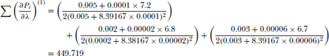
Now, the increment required for λ is:

The updated value of λ is:

 

 

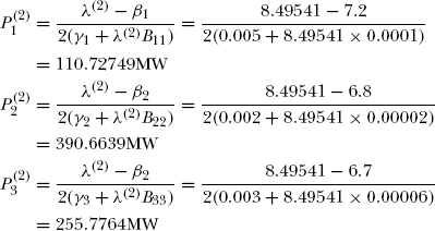
Third iteration:

With updated value of λ, the new generations can be obtained by using Eq.(2.24) as:

Loss at these generations is:

 

P_L = 0.0001 × 110.72749² + 0.00002 × 390.6639² + 0.00006 × 255.7764²

    = 8.2037MW

 

The error in the energy balance equality constraint is:

 

ΔP⁽²⁾ = 750 + 8.2037 − 110.72749 − 390.6639 − 255.7764

        = 1.03591MW

 

Using Eq.(2.30),

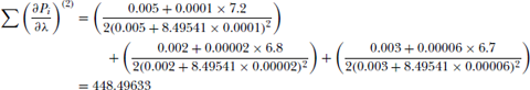
Now the increment for λ is:

The updated value of λ is:

 

                λ⁽³⁾ = λ⁽²⁾ + Δλ⁽²⁾ = 8.49541 + 2.30974 × 10⁻³

                      = 8.49771Rs/MWh

 

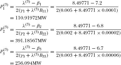
Fourth iteration:

With updated value of λ, the new generation can be obtained by using Eq.(2.24) as:

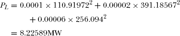
Loss at this generation is:

Error in the energy balance constraint is:

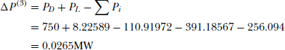
Since the error is small, the final optimal power flow solution can be taken as

 

                P₁ = 110.91972MW;    P₂ = 391.18567MW

                P₃ = 256.094MW;    P_D = 750MW;

                P_L = 8.22589MW