4.2 MODELLING OF TURBINE SPEED-GOVERNOR CONTROLLER

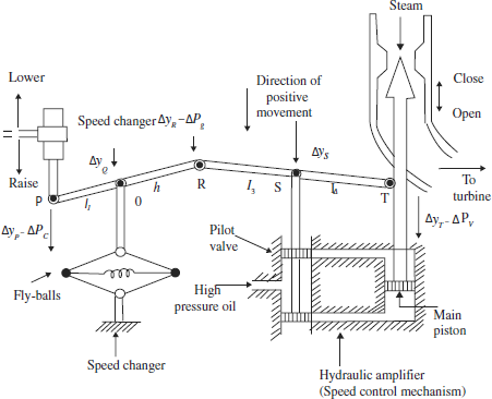
Fig. 4.2 is the schematic representation of a turbine speed governing system. It has four major components.

Speed governor: The Speed governor senses the change in speed (or frequency) and hence it can be regarded as heart of the system. The standard model of a speed governor operates by the fly-ball mechanism. Fly-balls moves outward when speed increases and the point Q on the linkage mechanism moves downwards, the reverse happens when the speed decreases. The movement of point Q is proportional to the change in shaft speed.

Linkage mechanism: PQR is a rigid link pivoted at Q and RST is another rigid link pivoted at S. This link mechanism provides a movement to the control valve in proportion to the change in speed. It also provides a feedback from the steam valve movement.

Hydraulic amplifier: It comprises of a pilot valve and main piston arrangement. It converts low power level pilot valve movement into high power level piston valve movement. This is necessary in order to open or close the valve towards high pressure steam.

Speed changer: It provides a steady state power output setting for the turbine. Its downward movement opens the upper pilot valve so that more steam is admitted to the turbine under steady conditions. The reverse happens for upward movement of the speed changer. By adjusting the linkage position of point P the scheduled speed frequency can be obtained for a given loading condition.

Mathematical Model of the Speed Governing System

Assume that the system is initially operating under steady conditions, the linkage mechanism is stationary and the pilot valve closed. The steam valve is opened by a definite magnitude, with the turbine running at a constant speed with turbine power output balancing the generator load

Let the operating conditions be characterized by

f⁰ = system frequency : p⁰_G = generator output; y⁰_T = steam valve setting

Let the point P on the linkage mechanism be moved downwards by a small amount ΔyP. It is a command which causes the turbine power output to change and can therefore be written as:

The command signal ΔP_c (i.e., ΔyT) sets into motion a sequence of events. The pilot valve moves upwards, high pressure oil flows on to the top of the main piston moving it downwards; the steam valve opening consequently increases and the turbine generator speed increases, i.e., the frequency goes up. Let us model these events mathematically.

Fig 4.2 Turbine speed governing system: Mathematical model of speed governing system

There are two factors which contribute to the movement of R:

1. Δyp contributes (or) −k₁Δ_yP (i.e upwards) of −k₁k_cΔP_c
2. Increase in frequency Δf causes the fly-balls to move outwards so that Q moves downwards by a proportional amount k₂ Δf, the consequent movement of R with P remaining fixed at Δ_yP is
   

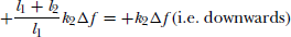
The net movement of R is therefore

The movement of S, Δys is the extent to which the pilot valve opens. It is contributed by ΔyR and Δyi. It can be written as

The movement Δys, depending upon its sign, opens the ports of the pilot valve admitting high pressure oil into the cylinder, thereby moving the main piston and opening the steam valve by ΔyT. The following justifiable assumptions are made:

1. Internal reaction forces of main piston and steam valve are negligible compared to the forces exerted on the piston by high pressure oil.
2. Because of (i) above, the rate of oil admitted to the cylinder is proportional to the port opening ΔyS. The volume of oil admitted to the cylinder is thus proportional to the time integral of ΔyS. The movement Δy_y is obtained by dividing the oil volume by the area of the cross-section of the piston. Thus
   

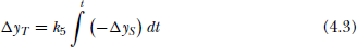
   From the Fig 4.2, we can conclude that a positive movement Δy_s, causes negative (upward) movement in ΔyT accounting for the negative sign used in Eqn. (4.3). Taking the Laplace transform of Eqns (4.1), (4.2) and (4.3).

   We get

    

   Δ Y_R(s) = −k₁k_cΔP_C(s) + k₂ΔF(s)                    (4.4)

    

   Δ Y_s(s) = k₃ΔY_R(s) + k₄ΔY(s)                        (4.5)
   

Substituting (4.4) in (4.5) and then in (4.6), we get by simplification

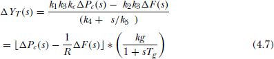
Where governor speed regulation. 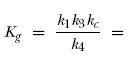gain of speed governor speed governor time constant

Figure 4.3 give the block diagram representation of Eq. (4.7)

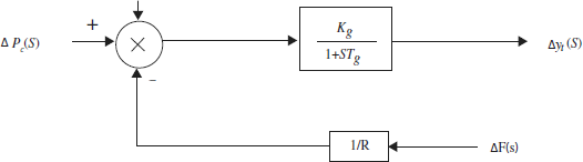
Fig 4.3 Block diagram representation of a speed governor