
In a previous recipe, we learned how to generate TikZ drawing commands from within gnuplot for inclusion in a LaTeX file. This recipe is, in a way, the reverse. We are going to learn how to generate gnuplot commands from within a LaTeX document.
The method introduced in this recipe is most useful when we want to enfold graphical elements into our typeset text rather than include them in floating figure environments. It also has the advantage of encompassing all the typesetting and drawing commands into a single file that is processed with one command, with no need to keep track of plot files and separate gnuplot scripts. This makes it simpler for your document source to become self-documenting and easily modifiable.
This is a flexible and powerful technique that allows us to combine plots generated by gnuplot with TikZ drawing commands. If we become proficient in TikZ, we will be able to arrange gnuplot graphs and PGF graphics in arbitrary ways on the page. As we don't have space here for a TikZ tutorial, we shall limit ourselves to the following simple example:
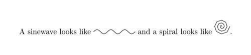
In the previous figure, we have a sentence typeset by LaTeX with some illustrations integrated into the line. The graphics were drawn by gnuplot and inserted back into the document by LaTeX, all automatically.
The technique we are going to learn now requires LaTeX, PGF, and gnuplot to work together to create a document with integrated text and graphics (PGF is the Portable Graphics Format, the actual drawing engine for which TikZ is a higher-level language). Unfortunately, there is an incompatibility between recent versions of gnuplot and all but the latest version of PGF. And, equally unfortunately, this latest version is not yet widely distributed. If, when trying this recipe, you see errors that complain about gnuplot not understanding "set term table" or something similar, then you need to upgrade your PGF installation. You can go to the official website at http://pgf.sourceforge.net/ and download version 2.10, and follow the install instructions. After the files are copied to the correct places in the TeX tree, you will need to run texhash as root (or administrator).
The following single LaTeX file creates the illustration shown in the previous figure:
documentclass{article}
usepackage{tikz}
usepackage{pgfplots}
usepackage[T1]{fontenc}
usepackage[utf8x]{inputenc}
pagestyle{empty}
egin{document}
A sinewave looks like 	ikzdraw[domain=0:18.84, scale=.1] plot func tion{sin(x)};
and a spiral looks like 	ikzdraw[parametric, domain=0:18.84, scale=.1]
plot function{.2*t*cos(t),.2*t*sin(t)};.
end{document}
This file must be processed with an extra argument to the pdflatex command that gives permission for the document to invoke an external program (in our case, gnuplot). This is for security; the concern is that malicious TeX documents might run programs without the user's knowledge, so you must turn on this ability manually. Usually, the command is pdflatex --shell-escape file, but on some systems it is pdflatex --write18 file (where, in both cases, you substitute the name of your TeX file for file, leaving off the .tex file extension).
This will work in any LaTeX document, but we must be sure to include the tikz and pgfplots packages. The highlighted lines create the sentence shown in the previous illustration. When it's time to insert our pictures, we start the ikz command, followed by draw with the options in square brackets. The domain option serves the same purpose as the [a:b] plot notation within gnuplot; the scale option scales the final figure by the multiplicative factor supplied; and the parametric option means that the following plot command is a parametric function, with t as the parameter and the x and y coordinates separated by a comma (we covered parametric plotting in Chapter 1,
A single command on our part is all that is required. LaTeX calls out to gnuplot automatically to create tables that are subsequently read in by PGF to create the illustrations, which are inserted into the page by the TeX typesetting engine. There will be a few auxiliary files left on the disc, which you can safely delete, but they may speed up subsequent passes through LaTeX if you are actively editing the file.
TikZ/PGF can produce any type of diagram, and TikZ pictures can be put inside of a floating figure environment, as we saw in the previous recipe. But where TikZ excels is the ease with which it can place small illustrations in line with the text. This can be done with the extensive graphical capabilities built into TikZ/PGF, which actually include the ability to make simple plots directly. As this is not a book about TikZ but about gnuplot, we've chosen to demonstrate how TikZ can use gnuplot as an external program. This is invoked with the function keyword in the highlighted line. If you want a full-blown graph with axes, tic marks, and so on, you can use other TikZ commands to create these, including LaTeX-typeset labels; but in this case you may be better off using the techniques of the previous two recipes.