
It is possible to plot a surface and its projection as a color image on the x-y plane on the same graph. The two simultaneous views of the same data or function can be useful to bring out the topography of a complex surface.
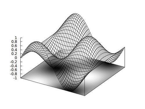
The previous figure shows a simple trigonometric function of two variables displayed as a surface with its values simultaneously encoded into colors (or gray values) at the base of the plot.
The following script produces the previous figure as its output:
set iso 40
set samp 40
unset key
set xrange [-pi:pi]
set yrange [-pi:pi]
f(x,y) = sin(x)*cos(y)
set hidden front
set xyplane at -1
splot f(x,y) with pm3d at b, f(x,y) with lines
The new features we are combining to produce this graph are in the highlighted lines in the code sample. Let's look at the last command first. The first part of the splot command plots the function f(), which is defined three lines above, as a colored surface at the base of the plot; this is what pm3d at b does. The second part, after the comma, plots the function again, without pm3d but with lines. This plots the wireframe surface.
The function varies from -1 to 1, but we want it to lie completely above the base upon which the surface is drawn, so we need to change the z value at which we place the base. This is the purpose of the second to last line.
Finally, we would like the surface to appear solid. But when combining surfaces with pm3d color plots, we need to add an extra option to the set hidden3d command, because the hidden line removal does not apply to the pm3d part of the graph. The command set hidden front tells gnuplot to draw the parts of the graph involving the hidden line removal procedure after the other parts, so they appear to be "in front" of the colored base, giving the effect we want.
We can make the image intersect the surface, as shown in the following:
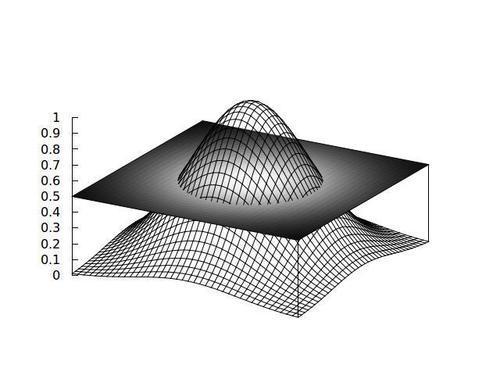
This is a simple 2D Gaussian surface cut through by the x-y plane, upon which the function's values are shown as colors or in grayscale. The code follows:
set samp 40
set iso 40
set yrange [-1.5:1.5]
set xrange [-1.5:1.5]
unset ytics
unset xtics
unset key
unset colorbox
set hidden3d front
a = .5
set xyplane at a
f(x,y) = exp(-x**2-y**2)
splot f(x,y) with pm3d at b, f(x,y) with lines, a with lines lt -100
We've taken advantage of the fact that we can place the base wherever we want to make it intersect the surface at a, which we've set to 0.5. But it's not quite so simple, as a little trick is required to make the color projection on the base to appear to be opaque; otherwise, we would be able to see the surface through it, which would make the graph confusing. Remember that hidden line removal does not work on the pm3d surface, so we need to add something else to the x-y plane to make it appear to be opaque. This is the purpose of the last part of the splot command, where we have asked for a plot of the constant value a using the linetype (lt) -100. As the global hidden3d option is turned on, this plot will be made using hidden line removal; and as we have specified a linetype that happens not to exist, the lines themselves will be invisible. The net result is a surface, invisible except for its ability to hide what is beneath it, having the constant value a, which will exactly coincide with the base of the plot.
We can also plot two different sets of data or functions, one used for the surface and the other for the image:
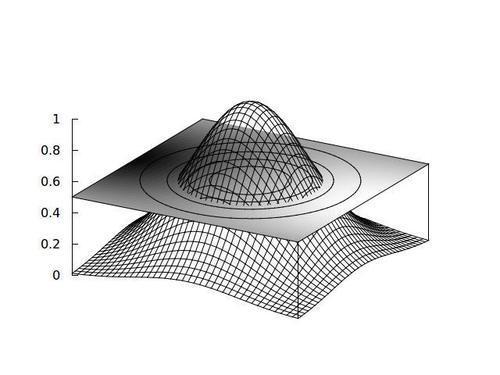
The previous plot retains the 2D Gaussian surface from before but plots a simple 2D trigonometric function in an image. For good measure, we've thrown in a contour plot as well. The plot was made with the following script:
set samp 40
set iso 40
set yrange [-1.5:1.5]
set xrange [-1.5:1.5]
set zrange [0:1]
unset ytics
unset xtics
unset key
unset colorbox
set hidden3d front
a = .5
set xyplane at a
set contour base
f(x,y) = exp(-x**2-y**2)
splot '++' using 1:2:(a):(sin($1)*cos($2)) with pm3d at b,
'++' using 1:2:(f($1,$2)) with lines, a with lines lt -100
By now, this should all be familiar, except for the last command. We've combined our previous tricks with the use of the "++" pseudofile in order to get different data used for the surface (and contours) and the image. This is the technique used earlier in this chapter in the Combining contours and images recipe.