
Back in Chapter 1, Plotting Curves, Boxes, Points, and more, we used parametric plotting to make graphs of complicated 2D paths. We can do the same thing in 3D to draw a complex curve in space.
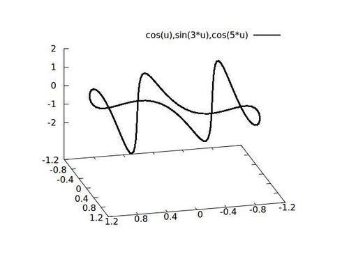
This might be thought of as a 3D Lissajous figure. The path intersects itself at several places.
Following is the code for the previous figure:
set samp 100
set xtics .4
set ytics .4
set parametric
set urange [-pi:pi]
set ztics 1
splot cos(u),sin(3*u),cos(5*u) lw 2
Note that the appearance of the plot will change radically depending on the viewpoint.
In exploring parametric plotting in 2D in Chapter 1, Plotting Curves, Boxes, Points, and more, we learned that the x and y independent variables were replaced by the single parameter t, and we had to specify two functions separated by commas; the first gave the x coordinate and the second gave the y coordinate that were plotted simultaneously as t was varied between the limits defined in the trange.
To plot a parametric curve in 3D, it may not come as a surprise that we need to specify three functions (or data columns) separated by commas. This can be seen in the last command of the previous script. When we give the command set parametric in 3D, two new independent variables u and v are established, which act as the parameters. We need to set their ranges, which we do here with the set urange command (we don't use v in this example, but we do in the next, when we explore parametric surfaces).