
We have learned how to use a large number of gnuplot commands and assembled them into scripts, included with this book as code samples, that can be executed from the command line or read in from the gnuplot's interactive plot with the load command. Up to now, however, these scripts have taken the form of a simple sequence of commands, each one to be executed once; the same result is obtained whether we enter the commands one at a time at the prompt or load the script as a whole, in batch mode.
There are many tasks that are much more convenient, and others that are only possible, if we can apply some sort of automation to the generation of commands. Fortunately, gnuplot, as part of its command language, includes a simple facility for applying some basic programming constructs. There is a basic looping control, a way to iterate over a set of commands, and an if—then—else statement. With these few borrowings from procedural languages, we can do a great deal; and, as we shall see later on in the chapter, if we need more, we can control gnuplot from within almost any general-purpose programming language. In the following figure, the Bessel function is plotted five times, each time with its argument scaled differently, with a different linetype for each curve, and with a curve title for the legend constructed individually for each plot:
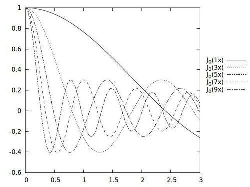
The previous graph could have been made by issuing five individual plot commands, but in fact was produced with a single line highlighted in the following gnuplot script:
set term pngcairo mono dashed enhanced
set out "file.png"
set rmargin at screen .8
set key at screen 1,.7
plot [0 : 3] for [n = 1 : 10 : 2] besj0(n*x) title "J_0(".n."x)" lt n
The selection of terminal type and output file in the first two lines may be familiar from previous chapters. This recipe will work for any terminal type, so these details are not crucial; however, we want to select enhanced text handling so we can use subscripts in the legend, and we've also specified dashed monochrome plot curves so the different lines can be distinguished in black and white output, as in the printed version of this book.
The highlighted line contains the new concept for this recipe: within the plot command is embedded a new construct. The for keyword introduces a loop iteration similar to the for loop in C and similar languages. The loop variable (in this case n) is introduced within the square brackets; the notation here means that n goes from 1 to 10 in steps of 2: 1, 3, 5, 7, 9. The plot command is repeated for each value of n, and wherever n appears in the command its value is substituted. The result is that this one compact line, highlighted in the script, is equivalent to the long, compound plot command:
plot [0 : 3] besj0(1*x) title "J_0(1x)" lt 1,
besj0(2*x) title "J_0(2x)" lt 2,
...
When constructing our curve titles, we've used the string catenation operator, which is a dot; when integers are joined with strings in gnuplot, the integers (the variable n here) are first typecast to strings.
We have enlarged the right margin with the set rmargin command, and specified a location for the legend with the set key command, using screen coordinates, to place the key outside the plot on the right. This is helpful when there are many curves in a plot that might collide with the legend.
The for loop is available in the plot command, as demonstrated in the previous script, and also in the set command, where it can be used, for example, to define a whole series of user linestyles (see Chapter 3, Applying Colors and Styles) all at once.
But gnuplot has a more flexible style of iteration that we can turn to when its simple for loop is not sufficient. This is accomplished with the use of the reread keyword in conjunction with an if statement, as shown in the following script:
plot sin(0.1*n*x)
n = n + 1
if (n < 100) reread
In order to use this code block, we must first save it in a file (the code has been included as a supplemental sample for this recipe). Start up gnuplot and get the interactive prompt. Then set the variable n to 1 by simply saying n = 1. If we wish, we can now set terminal and other options; let's set the terminal to one of the onscreen terminals such as X11 or wxt, and say set samples 1000 for a smooth plot. Now, if we say load file, substituting the name of the file where we saved the previous code sample, we should see a nice animation of a sine wave sweeping from a low to a high frequency.
This happens because of the final (highlighted) line. The last word on that line, reread, is a special keyword that tells gnuplot to go back to the beginning of the file and execute it again. But each time the file is loaded, the value of n is incremented by the second line, and it is retained. This could continue forever, but is terminated by the if clause, which only executes the reread when n is less than 100. Instead of displaying an animation on the screen, we could have saved each plot to a separate file by incorporating the n variable into a filename using the string catenation operator (set out "file".n."png" would do it). Then, we could use any of a number of programs to stitch the files together into a movie. In this way, gnuplot's simple iteration facilities can be used to create animations for presentations or teaching. The recipe Creating presentation slides with incrementally displayed graphs in Chapter 6, Including Plots in Documents contained a script that produced a series of graphs for inclusion into a presentation. Using the looping technique introduced in this recipe, we can now see how this script could be written more concisely, and with less chance for typos to creep in.