15
Aircraft Performance
15.1 Overview
This is the culminating chapter to assess if the sized aircraft configured, thus far, meets the Federal Aviation Regulation (FAR) requirements and the customer specifications. Classroom work follows in a linear manner from the mock market survey (Chapter 2). The requirements and the specifications dealt with in this chapter comprise of aircraft performance to substantiate the (i) takeoff and (ii) landing field lengths (LFLs), (iii) initial rate of climb, (iv) maximum speed at initial cruise and, especially for civil aircraft design, its (v) payload range plus (vi) the turn rate for the Advanced Jet Trainer (AJT). Chapter 18 computes aircraft Direct Operating Cost (DOC), which should follow the aircraft performance estimation.
Aircraft performance is a subject all on its own. All aeronautical schools offer the subject as a separate course. Therefore, to substantiate the FAR and customer requirements, this chapter deals only with what is required, that is, the related governing equations and examples associated with the items listed above. Note that substantiation of payload‐range requires integrated climb and descent performances showing fuel consumed, distance covered and time taken for the flight segments. Readers are recommended to refer to [1] by the authors, as a companion book, dealing with the same aircraft performance in extensive details. The turboprop example is not worked out but there is enough information to compute it in a similar manner.
The rest of the book beyond this chapter has information that aircraft designers should know and apply.
The chapter covers the following
- Section 15.2: Introduction
- Section 15.3: Takeoff Performance
- Section 15.4: Landing Performance
- Section 15.5: Climb Performance
- Section 15.6: Descent Performance
- Section 15.7: Initial Maximum Cruise Speed Capability
- Section 15.8: Payload‐Range Capability
- Section 15.9: In Horizontal Plane (Yaw Plane) – Sustained Coordinated Turn
- Section 15.10: Aircraft Performance Substantiation – Bizjet
- Section 15.11: Aircraft Performance Substantiation – AJT
- Section 15.12: Propeller‐Driven Aircraft Performance Substantiation – TPT
15.1.1 Section 15.13: Summarised Discussion of the DesignClasswork Content
At this stage of project design, only the substantiation of requirements/specifications are required for the sized aircraft configurations culminating in ‘concept finalisation’ as worked out in Chapter 14. Full aircraft performance for the full envelope is carried out after go‐ahead is obtained, as done in [1] by the same authors.
The readers will have to compute the following for their projects. This follows that the readers have made engine performance available as shown in Sections 13.4 and 13.5.
- Substantiate the takeoff field length (TOFL). This has to demonstrate that the aircraft is capable of meeting the Federal Aviation Administration (FAA) second segment (see Figure 15.3) climb gradient requirement for the most critical case.
- Substantiate the initial climb rate. This is not a FAA requirement but a market specification.
- Substantiate the initial high speed cruise (HSC) capability. This is also not a FAA requirement but a market specification.
- Substantiate the LFL. This has to demonstrate that the aircraft is capable of meeting the FAA requirement for the most critical case.
- Substantiate the payload‐range capability. This is also not a FAA requirement but a market specification. Payload‐range computation requires the specific range, integrated climb and descent performance of the aircraft and the readers will have to compute these. Use of spreadsheets is recommended.
For the trainer aircraft, the following are the additional requirements.
- Compute turn capability. This is not a Milspec requirement but a MoD (Ministry of Defence) specification.
- Compute the training mission profile to substantiate the capability.
If any of the aircraft performances is not met then aircraft has to be configuration iterated (see Chapter 8 up to Chapter 14) until the requirements are met. The spreadsheet method proves convenient for iteration.
Airworthiness regulations differ from country to country. Military certification standards are different from the FAA. In the USA, this is guided by Milspecs. Certification authorities have mandatory requirements to ensure safety at takeoff and landing. For further details on respective certification regulations, the readers may refer to their official websites. Readers are recommended to read references 2–8 for supplementary coverage.
15.2 Introduction
The final outcome of any design is to substantiate aircraft performance for what it is intended to do. In the conceptual design phase, aircraft performance substantiation needs to be carried out mainly on those critical areas as required by the FAR and also customer requirements. Full aircraft performance estimation is done subsequently (beyond the scope of this book). All worked out aircraft performance estimations are done at a standard (STD) day. Non‐International Standard Atmosphere (ISA) day performance computations are done in the same way with non‐ISA day data.
The sizing exercises in Chapter 14 showed a rapid performance method to generate the relation between wing loading, W/SW, and thrust loading, TSLS/W, to obtain the sizing point that would simultaneously satisfy the requirements of takeoff/LFLs, initial rate of climb capability and maximum speed at initial cruise. The aircraft sizing point gives the installed maximum sea level takeoff static thrust, TSLS of the matched engines.
Chapter 13 gives generic uninstalled engine performances of rubberised engines in a non‐dimensional form, from which installed thrust and fuel flow rates at various speeds and altitudes at the power settings of takeoff, maximum climb and maximum cruise ratings by STD day are worked out in Sections 13.4 and 13.5. Using these installed engine performance data, this chapter continues with a more accurate computation of aircraft performance to substantiate the specified takeoff and LFLs, initial rate of climb, maximum speed at initial cruise and payload range. At this point, it may be necessary to revise aircraft configuration if the performance capabilities are not met. If the aircraft performance indicates shortfall (or excess) in meeting the requirements, then the design is iterated for improvement. In classroom work, normally one iteration should prove sufficient, but the readers should not hesitate to fine‐tune with iterations; it is a normal industrial practice.
Finally, at the end of the design, the aircraft should be flight tested over the full flight envelope including various safety issues to demonstrate compliance. This concludes concept finalisation as the obligation of this book.
15.2.1 Aircraft Speed
Aircraft speed is a vital parameter in computing performance. It is measured from the difference between the total pressure, pt and static pressure, ps, expressed as (pt − ps). Static pressure is the ambient pressure in which the aircraft is flying and the total pressure, pt, is aircraft speed dependent. The value of (pt − ps) gives the dynamic head, which depends on the ambient air density ρ and aircraft velocity (speed). Unlike automobile ground speed measured directly, aircraft ground speed needs to be computed from (pt − ps). The pilot reads the gauge reading converted from (pt − ps). The following are the various forms of aircraft airspeeds that engineers and pilots use. As can be seen, these require some computations – nowadays onboard computers do it all.
- Vi = Gauge reading is what the uninstalled bare instrument supplied by the manufacturer reads. The instrument includes standard adiabatic compressible flow corrections for high subsonic flight at a sea level STD day. But it still requires other corrections as follows:
- VI = Indicated Airspeed (IAS). Manufactured instruments will have some built‐in instrumental errors, ΔVi, (normally very small but an important consideration when close to stall speed). Instrument manufacturers supply the error chart for each instrument. The instrument is calibrated to read correct ground speed at sea level STD day with compressibility corrections. When corrected the instrument reads IAS.

- VC = Calibrated Airspeed (CAS). Instrument manufacturers calibrate the uninstalled bare instrument for sea level conditions. Once installed on an aircraft, depending where it is installed, the aeroplane flow field will distort instrument readings. Therefore, it will require position error (ΔVp) corrections by aircraft manufacturers.

- VEAS = Equivalent Airspeed (EAS). Air density ρ changes with altitude – it goes down because atmospheric pressure reduces with gain in altitude. Therefore, at the same ground speed (also known as True Air Speed, TAS), the IAS would read lower values at higher altitudes. The mathematical relation between TAS and EAS reflecting the density changes with altitude can be derived as TAS = EAS/√σ, where σ is the density ratio (ρ/ρ0) in terms of sea level value, ρ0. A constant EAS has a dynamic head invariant. For high subsonic flights, it will require an adiabatic compressibility correction (ΔVc) for the altitude changes.

VEAS is what the pilot in the flight deck reads. In the past, the pilot/flight engineer had to manually correct the instrument and position errors. Today, these corrections are embedded in the aircraft microprocessors off‐loading manual effort.
Compressibility corrections for position errors is also there but at this stage such details can be avoided without any loss of conceptual design work undertaken in this book. Supersonic flight will require further adjustments to make the corrections resulting from the shock wave associated with it.
15.2.2 Some Prerequisite Information
The readers will have to find available engine performance data, as done in Chapter 13 in which the installed thrust and fuel flows for the various engines are worked out. The worked‐out examples in this chapter uses the following figures.
- Turbofan with a BPR (bypass ratio) ≈ 4 ± 1, (in the class of Honeywell TPE731 turbofan) – Bizjet application
- Figure 13.11 – Installed takeoff thrust and fuel flow per engine
- Figure 13.12 – Installed maximum climb thrust and fuel flow per engine
- Figure 13.13 – Installed maximum cruise thrust and fuel flow per engine
- Figure 13.14 – Installed idle engine thrust and fuel flow per engine
- Military Turbofan with a BPR < 1, (in the class of Rolls‐Royce/Turbomeca Adour) – AJT application
- Figure 13.15 – Installed maximum thrust and fuel flow for all the three ratings.
- Turboprop engine, in the class of Garrett TPT 331 – TPT application
- Figure 13.16 – Installed takeoff thrust and fuel flow per engine
- Figure 13.17 – Installed maximum climb thrust and fuel flow per engine
- Figure 13.18 – Installed maximum cruise thrust and fuel flow per engine
Using the engine and aircraft data obtained thus far during the conceptual design phase, this chapter checks whether the configured aircraft satisfies the airworthiness (FAR) requirements and the customer specifications in the takeoff/landing, the initial climb rates and the maximum initial cruise speed plus the payload‐range capability (civil aircraft).
15.2.3 Cabin Pressurisation
Aircraft payload‐range computation requires integrated climb and descent performances. It is topical to introduce the role of cabin pressurisation in assessing aircraft climb and descent performance. Ambient pressure reduces non‐linearly with increase in altitude as can be seen in Figure 1.8. At the tropopause it is 472.68 lb ft−2 (3.28 lb in−2). For average human physiology, big jets maintain cabin pressure around 8000 ft altitude (ambient pressure of 1571.88 lb ft−2 (10.92 lb in−2) resulting in a differential pressure of 7.63 lb in−2). Smaller Bizjets fly at higher altitudes to stay separate from big‐jet traffic, as high as 50 000 ft altitude (242.21 lb ft−2, i.e. 1.68 lb in−2) when aircraft structural design considerations are made to maintain the inside cabin pressure at 10 000 ft altitude (1455.33 lb ft−2, i.e. 10.11 lb in−2, a differential pressure of 8.42 lb in−2). For big jets, a maximum of 8.9 lb ft−2 (for Bizjets to 9.4 lb in−2) of differential pressure is used in practice. Cabin pressurisation is in use for certain types military aircraft with large fuselage volumes. Combat aircraft have different arrangements for higher altitude provision in the flight deck; pilots wear pressure suits and helmets with masks supplying them with oxygen.
The differential pressure between the outside and inside of the cabin is substantial and it cycles through every sortie flown. Stress and fatigue considerations of fuselage structural design are constrained by weight considerations. Aircraft cabins are built as sealed pressure vessels (very low leakage), kept airtight and provided with complex environment control systems (ECSs), which have pressure control valves to automatically regulate cabin pressure (and air‐conditioning). The aircraft crew can select the desired cabin pressure within the design limits. Unless there is a catastrophic failure, the sealed cabin can hold pressure to give enough time for pilots to descend fast enough in case there is a malfunction in pressurisation. If cabin pressure exceeds the limit then automatic safety valves can relieve cabin pressure to bring it down within safe limits.
The classwork example of the Bizjet has cabin pressure selectable from sea level to 10 000 ft altitude, limiting the differential pressure to within 9.4 lb ft−2. During the climb the equivalent Bizjet cabin pressure rate of change is designed to 2600 ft min−1. Bizjet type aircraft engine power is adjusted to have cabin pressurisation at the climb rate to a maximum of about 1800 ft min−1 to stay within the ECS system capability, sufficient for the sealed cabin that starts with sea level pressure, and as a result en route climb rate is not required to be restricted. Section 15.10.5 works out the Bizjet climb performance. However, during descent, the cabin needs to gain pressure as it descends to lower altitudes. Average human physical tolerance is taken at 300 ft min−1 descent and the ECS system pressurisation capability meets that.
The following equations are derived in this chapter.
- TOFL equations
- Climb and descent equations
- Cruise equations
- LFL
- Range equations to establish the payload‐range capability
- Aircraft turn equations
15.3 Takeoff Performance
At takeoff, the ground run is initiated with an aircraft under maximum thrust (takeoff rating) to accelerate, gaining speed until a suitable safe speed is reached when the pilot initiates rotation of the aircraft by gently pulling back the control stick/wheel (elevator going up) for lift‐off. In the case of an inadvertent situation of the critical engine failure, provision is made to cater for safety so that the aircraft can continue with its flight and return immediately to land.
While regression can analyse from the data statistics within the class of aircraft to generate semi‐empirical relations that can yield close enough results, they mask the understanding of the physics involved in the takeoff procedure to estimate Balanced Field Length (BFL) (see Figure 15.2) with one engine inoperative. The mandatory certification regulations require complying with specified speed schedules and the determination of the decision speed, V1, in case of one engine failed, are not captured in the semi‐empirical relations. It is for this reason that the authors think it is essential to adopt the formal procedure as practised in industry, except that the treatise is relaxed with simplifications for classroom usage. For example, there is no easy way to determine the CL and CD of aircraft in the transient state of operation during a takeoff ground run with speed accelerating but not yet airborne. In this book, average values are taken where necessary. Industries have computer programs to accurately estimate BFL in all ambient conditions that also establish the relation between aircraft weight, airfield altitude and ambient temperature (WAT: weight, altitude and temperature) and their limitations for operational use in all‐weather conditions [1]. Takeoff analysis is one of the more involved methods and the readers must perform manual computation for, at least, one set of analysis to appreciate the procedure and assess the labour content, then use a spreadsheet as a labour saving option.
Designers must know the sequence of the takeoff speed schedules stipulated by certification agencies (Figure 15.1). To ensure safety, certification authorities demand a mandatory requirement to cater for taking off with one engine inoperative to clear a 35 ft height representing an obstacle. A one engine inoperative TOFL is computed by considering the BFL when the stopping distance after an engine failure at the decision speed, V1, is the same as the distance taken to clear the obstacle at maximum takeoff mass (MTOM) (Figure 15.1). The speed schedule is related to Vstall, a known value for the sized MTOM and type of high‐lift device incorporated. These are explained next.
- V1: This is the decision speed. An engine failure below this speed would result in the aircraft not being able to satisfy takeoff within the specified field length, but it will be able to stop. If an engine fails above the V1 speed, the aircraft should continue with the takeoff operation.
- Vmc: This is the minimum control speed at which the rudder is effective to control the asymmetry created by one engine failure. This should be lower than the decision speed, V1, otherwise at the loss of one engine the aircraft cannot be controlled if continuing with takeoff.
- VR: This is the speed when the pilot initiates the action to rotate the aircraft for lift‐off. VR should be more than 1.05 Vstall. Once this is done, reaching VLO and V2 occurs as a fall‐out of the action.
- Vmu: There is a minimum unstick speed, above which the aircraft can be made to lift off. This should be slightly above VR. In fact, Vmu decides VR. If the pilot makes an early rotation then Vmu may not be sufficient for lift‐off and the aircraft will tail drag until it gains sufficient speed for the lift‐off.
- VLO: This is the speed at which the aircraft lifts off the ground and it is closely associated with VR. In a case of one engine being inoperative, it should be VLO ≥ 1.05 Vmu.
- V2: This is the takeoff climb speed at 35 ft height, also known as the first segment climb speed. It is also closely associated with VR. FAR requires that V2 = 1.2 Vstall (at least – it can be higher).
- VB: This is the brake application speed at one engine failure (VB > V1).
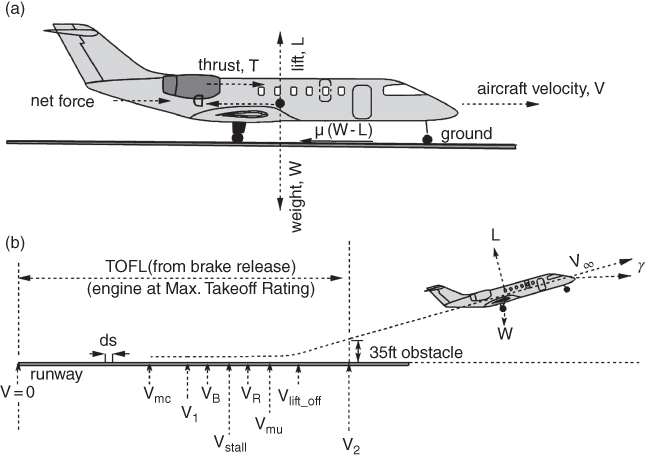
Figure 15.1 Takeoff, first and second segment climb (see Figure 15.3). (a) Takeoff forces and (b) takeoff ground run.
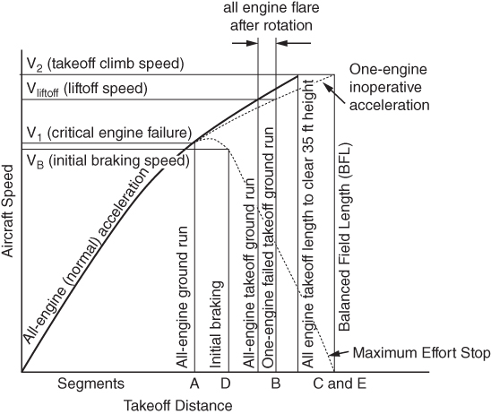
Figure 15.2 Balanced field length consideration.
15.3.1 Civil Transport Aircraft Takeoff [FAR (14CFR) 25.103/107/109/149]
To ensure safety, the takeoff procedure must satisfy the airworthiness requirement so that the aircraft will be able to climb to safety or stop safely in a case where one critical engine has failed. FAR (14CFR) 1.1 defines the ‘critical engine’ whose failure would most adversely affect aircraft takeoff procedure. Evidently, the most outboard engine of a multi‐engine aircraft is the critical one. Designing for critical engine failure also covers the safety aspects of the failure of a non‐critical engine for an aircraft with more than two engines.
Certification authorities demand mandatory requirements to cater for taking off with one engine inoperative to clear a 35 ft height representing an obstacle and continue with the required climb gradient (Figure 15.3). One engine inoperative TOFL is computed by considering BFL(Section 15.3.2) when the stopping distance after an engine failure at the decision speed, V1, is the same as the distance taken to clear the obstacle at MTOM.
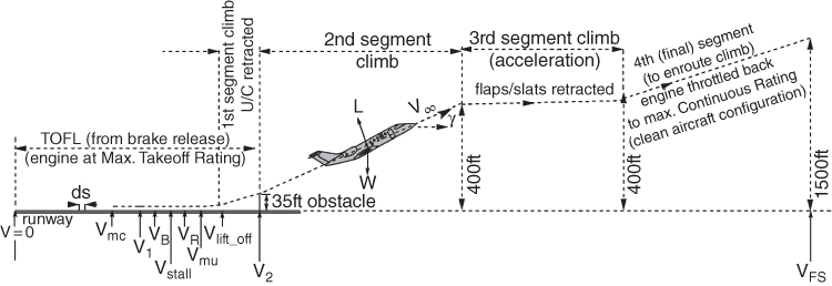
Figure 15.3 Takeoff, first, second, third and fourth segment climb (FAA).
FAR (14CFR) 25 requires takeoff substantiation for the both dry and wet runways. This book deals only with the dry runway considerations.
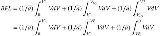
15.3.2 Balanced Field Length (BFL) – Civil Aircraft
The rated TOFL at MTOM is determined by the BFL in the event of an engine failure. Figure 15.2 shows the segments involved in computing BFL. It can be seen that taking off with one engine inoperative (failed) above the decision speed V1 has three segments to clear 35 ft height. Designers must provide the decision speed V1 to pilots below which, if an engine fails, then the takeoff has to be aborted for safety reasons. The BFL segments are defined next:
- Segment A. The distance covered by all engines operating a ground run until one engine fails at the decision speed V1.
- Segment B. The distance covered by one engine inoperative acceleration from V1 to VLO.
- Segment C. Continue with the flare distance from lift‐off speed VLO to clear the 35 ft obstacle height reaching aircraft speed V2.
In the case of engine failure, past the decision speed V1, there are two segments (which replace segments B + C), as follows.
- Segment D. The distance covered during the reaction time for the pilot to take braking action after an engine fails. (Typically, 3 s is taken as the pilot recognition time and brakes to act, spoiler deployment etc. At engine failure the thrust decay is gradual and within this reaction time before brake application there is a small speed gain shown in the diagram.) Typically, (VB ≥ V1) but can be taken as (VB ≈ V1).
- Segment E. Distance to stop from VB to V0 (maximum brake effort).
15.1

15.3.2.1 Normal All‐Engine Operating (Takeoff) – Civil Aircraft
Normal takeoff with all engines (TOFLall_eng) operating will take considerably lower field length than the one engine failed case (TOFL1eng‐faled). To ensure safety, FAR (14CFR) requires a 15% allowance is added to TOFLall_eng over the estimated value. Therefore, it must be at least equal to the greater of the two as shown next.
15.3.2.2 Unbalanced Field Length (UBFL) – Civil Aircraft
At low aircraft weights, the decision speed V1 at one engine inoperative can become lower than Vmc. Since V1 should not be below Vmc resulting in unbalanced field length (UBFL) as segments (B + C) < Segments (D + E). In this case, the TOFL is taken as segments (A + D + E). In another situation where V2 < 110% of Vmc it makes UBFL when the TOFL is taken as segments (A + B + C). UBFL is not computed in this book as it is not a specification/requirement at the conceptual design phase.
15.3.3 Civil Aircraft Takeoff Segments [FAR (14CFR) 25.107 – Subpart B]
A takeoff process with one engine inoperative (FAR requirement) can be divided into four segments (Figure 15.3) of climb procedure as follows:
| first segmenta | Climb to 35 ft, undercarriage retracting. |
| second segmenta | Climb from 35 to 400 ft undercarriage retracted. Engine power is kept at maximum takeoff rating. Drag reduction on account of undercarriage retraction is substantial. |
| third segment | In this segment the aircraft stays at 400 ft altitude to accelerate to higher speeds (V2 > 10 kt) to increase stall speed margin. The aircraft is at a clean configuration. |
| fourth segment | This is the final segment under the takeoff procedure: continues with one engine inoperative and the aircraft must land immediately at a designated airfield. With all engines operating the aircraft continues to accelerate to en route climb at a specified speed schedule. Engine is throttled back to maximum continuous rating. Aircraft speed reaches final segment velocity, VFS, to continue with the en route climb. |
undercarriage retraction starts as soon as a gradient is established and completes at a height above 35 ft, and can be seen within the first segment by the International Civil Aviation Organization (ICAO) requirement. FAR second segment climb is taken from 35 ft, a known height, as the undercarriage is retracted. The operational takeoff requirements by ICAO are in more detail than the design requirements governed by the FAA.
The capability at the end of the fourth segment is a customer requirement and not a FAR requirement. Tables 15.1 and 15.2 provide the aircraft configuration and power settings at the aircraft takeoff segment FAR requirement.
Table 15.1 Civil aircraft takeoff segment requirements and status (FAR (14CFR) 25.121 Subpart B).
| first segment | second segment | third segment | fourth segment | ||
| Altitude – ft | 35 to u/c retract | Reach 400 ft | Level at 400 ft | Reach 1500 ft | |
| Speed (reference) | Vlift‐off | V2 | V2 + 10 kt | V2 + 10 kt | |
| Engine rating | Max. Takeoff | Max. Takeoff | Max. Cont. | Max. Cont. | |
| Undercarriage | Retracting | Retracted | Retracted | Retracted | |
| Flaps/slats | Extended | Extended | Retracting | Retracted | |
| Max. climb gradient (%) | two‐engine | 0.0 | 2.4 | 0 | 1.2 |
| three‐engine | 0.3 | 2.7 | 0 | 1.5 | |
| four‐engine | 0.5 | 3.0 | 0 | 1.7 | |
The first segment speed schedules are interrelated and expressed in terms of the ratios of Vstall as given in Table 15.2. The range of velocity ratios in Table 15.2 are typical and could deviate a little so long as the FAR (marked with * in the table) stipulation is complied with.
Table 15.2 Civil aircraft first segment speed schedule.
| Two‐engine | Three‐engine | Four‐engine | |
| Percentage loss at an engine failure | 50 | 33.3 | 25 |
| Minimum climb gradient at first segmenta | 0% | 0.3% | 0.5% |
| Minimum climb gradient at the second segment a | 2.4% | 2.7% | 3% |
| VLO/Vstall (approx..) | 1.12–1.14 | 1.15–1.16 | 1.17–1.18 |
| VR/Vstall (approx..) | 1.1–1.18 | 1.14–1.18 | 1.16–1.18 |
| Vmu/VR (approx..) | 1.02–1.04 | 1.02–1.04 | 1.02–1.04 |
| V1/VR (approx.) | 0.96–0.98 | 0.93–0.95 | 0.9–0.92 |
| Vmc/V1 (approx..) | 0.94–0.98 | 0.94–0.98 | 0.94–0.98 |
| V2/Vstall | ≥1.2 | ≥1.2 | ≥1.2 |
aRefers to FAR stipulation.
Note that some engines at their takeoff rating can have augmented power rating (APR) that could generate 5% higher thrust than the maximum takeoff thrust for short period of time. These types of engines are not considered in this book.
It may be noted that only Vstall is determined from aircraft weight and CLmax and FAR requires that V2 ≥ 1.2 Vstall. All other speed schedules are interrelated with regulation requirements. At the conceptual design stage, the ratios are taken from the statistics of past designs and as the project progresses these are refined, initially from wind‐tunnel tests and finally from flight tests. Table 15.3 gives the important speed schedule ratios.
Table 15.3 Airworthiness regulations at takeoff.
| Civil aircraft design | Military aircraft design | ||
| FAR23 | FAR25 | MIL‐C5011A | |
| Obstacle height at V2 ft | 50 | 35 | 50 |
| Takeoff climb speed at 35 ft height V2 | ≥1.2 Vstall | ≥1.2 Vstall | ≥1.2 Vstall |
| Lift‐off velocity, VLO | ≥1.1 Vstall | ≥1.1 Vstall | ≥1.1 Vstall |
| TOFL (BFL) | |||
| One engine failed | As computed | As computed | As computed |
| All engines operating | as computed | 1.15 × as computed | as computed |
| Rolling coefficient, μ | not specified | not specified | 0.025 |
Performance engineers must know the sequence of the takeoff speed schedules stipulated by certification agencies as given in Table 15.4.
Table 15.4 Civil aircraft takeoff speed schedule (FAR requirements).
| All‐engine operating | One engine inoperative | |||||
| Speed schedule engine | Two‐engine | Three‐engine | Four‐engine | Two‐engine | Three‐engine | Four‐engine |
| V2/Vstall | ≥1.20 | ≥1.20 | ≥1.20 | ≥1.20 | ≥1.20 | ≥1.20 |
| VLO/Vmu (approx.) | ≥1.10 | ≥1.10 | ≥1.10 | ≥1.05 | ≥1.05 | ≥1.05 |
| VR/Vmc (approx.) | ≥1.05 | ≥1.05 | ≥1.05 | ≥1.05 | ≥1.05 | ≥1.05 |
VR is selected in such a way (from past experience subsequently finalised by flight tests) that it reaches V2 speed at 35 ft altitude. Much depends on how the pilot executes rotation; FAR gives the details of requirements between maximum rate and normal rates of rotations. From the FAR requirements it can be seen (Figure 15.1) that V2 > VLO > Vmu > VR > Vstall > V1 > Vmc.
The higher the thrust loading (T/W), the higher the aircraft acceleration. For small changes, VR/Vstall and VLO/Vstall may be linearly decreased with an increase in T/W. The decision speed V1 with an engine failed is established through iterations as shown in Section . In a family of derivate aircraft, the smaller variant can have V1 approaching values close to VR.
Military aircraft requirements (MIL‐C5011A) are slightly different from the civil requirements. The first segment clearing height is 50 ft instead of 35 ft. Many military aircraft have a single engine where the concept of BFL is not applicable. Military aircraft have to satisfy the Critical Field Length (CFL) as described in Section 15.11.2. The second segment rate of climb is to meet a minimum of 500 ft min−1 for multi‐engine aircraft.
15.3.4 Derivation of Takeoff Equations
The derivation of takeoff performance equations is done at sea level STD day, an airfield with no gradient, zero wind conditions and thrust is aligned along the flight path (i.e. no thrust vectoring). The generalised equation for takeoff performance is derived in detail in [1].
15.3.4.1 Acceleration
Let the acceleration of the aircraft be denoted by a. The force balance equation resolved along aircraft velocity vector is given next (Figure 15.1).
Net force on the aircraft, (W/g)a = ΣApplied forces along aircraft velocity vector = ΣFapplied
where, V and a are instantaneous velocity and acceleration of the aircraft
Rearranging Eq. 15.3,
In terms of coefficients and rearranging (all‐engine operating)
A simplified approach can be taken by taking average acceleration ā for aircraft at 0.707 VLO (average of VLO2 from zero, that is, at √(VLO2/2) of the following equation). Then

where SW is the wing area and q = 0.5ρV2 is the dynamic head.
The aircraft on the ground encounters rolling friction (coefficient μ = 0.025–0.03 for a paved, metalled runway). At braking friction, μB = 0.3–0.5 (for the Bizjet, it is taken as 0.4). Thrust loading (T/W) is obtained from the sizing exercise. Average acceleration, ā, is taken at 0.707 VLO. FAR requires V2 = 1.2 Vstall. This gives V22 = [2 × 1.44 × (W/SW)]/(ρCLstall). An aircraft stalls at CLmax.
15.3.4.2 Takeoff Field Length (TOFL) Estimation – Distance Covered from zero to V2
Figures 15.1 and 15.2 show that aircraft is under all‐engine operation up to the decision speed, V1, and, thereafter, if the decision is made, continues with the takeoff procedure: the aircraft is rotated at VR to flare out and have lift‐off at VLO to reach to V2 to climb to a 35 ft altitude. It takes about 3–4 s time to reach V2 from VR. If aborted at V1, then the aircraft is braked to stop.
Form Figure 15.1, let dS be the elemental ground run distance covered by the aircraft in infinitesimal time dt. If the instantaneous velocity of the aircraft at that point is V then.
Then the distance, S, covered from the initial velocity Vi = 0 to final velocity, Vf, is obtained by integrating Eq. . Aircraft acceleration and engine thrust varies with aircraft speed. At the conceptual stage of design, taking average values would prove convenient. Taking average acceleration ![]() as a constant and using Eq. 15.7, the equation for distance, S, can be written as follows.
as a constant and using Eq. 15.7, the equation for distance, S, can be written as follows.

For initial velocity Vi ≠ 0 the ground run, Eq (15.8) can be re‐written in terms of the average condition as follows.

where using Eq. 15.5, the average acceleration can be written in coefficient form as follows
ā = {g [(T/W – μ) – (CLSq/W)(CD/CL – μ)]}ave (in System International (SI) units ‘g’ drops out).
Equation (15.8) can now be written separately for each segment and then equated for the BFL. The average acceleration ā is of the segment. A simplified approach can be taken by taking average acceleration ā for aircraft at 0.707 ΔV (average of ΔV within the velocity interval, at √(ΔV2/2) of the following equation).

In case it is aborted, the distance, Sabort, covered is as follows.

For the BFL,
The proper choice of the decision speed V1 will give the BFL. A number of iteration may be required to arrive at the proper V1, as shown in the classroom example in Section 15.10.1.2.
(In later stages of the project, the computation could be done more accurately in smaller steps of speed increment within which average values of the variables are considered as constants. During takeoff, aircraft CL and CD vary with speed changes. In the worked‐out examples, average values are taken. Reference [1] describes the takeoff procedure in detail.)
During takeoff, FAR requires V2/Vstall > 1.2. The speed gain continues during the rotational (VR) through aircraft flaring out to V2. In this phase, typically around 5% change occurs in aircraft velocity through acceleration at the most critical condition; it amounts to about a 5–7 kt speed increase. Therefore, only the proper choice of the decision speed V1 will give the BFL. A number of iterations may be required to arrive at the proper V1, as shown in the classroom example in Section 15.7.
Given next are the typical takeoff speeds V2 (with high‐lift device deployed) for some of the larger jet transport currently in operation.
| Boeing737: 150 mph | Boeing747: 180 mph | Airbus320: 170 mph |
| Boeing757: 160 mph | Concorde: 225 mph | Airbus340: 180 mph |
15.4 Landing Performance
Computation of LFL uses a similar equation as for computing the TOFL. The difference is that landing encounters deceleration, that is, negative acceleration. Typically, the engine(s) runs idle producing no thrust. Values of friction coefficient, μ, vary at main wheel touch down, then when the nose wheel touches down and when the brakes are applied after nose wheel touchdown (taken here as 2–3 s after touchdown). A considerable amount of heat is generated at full braking and may pose some fire hazard. If brake parachutes are deployed then the drag of the parachute is to be accounted for in the deceleration. With a thrust reverser, the negative thrust needs to be taken into account as the decelerating force. With full flaps extended and with spoilers activated, the aircraft drag is substantially higher than at takeoff.
The landing speed schedules and landing procedure are given in Figure 15.4. Landing performance estimation is carried out at ISA day, sea level, with zero wind and on an airfield without gradient. The landing configuration is with full flaps extended and the aircraft at its landing weight. The approach segment at landing is from 50 ft altitude to touch down. At approach, the FAR requires that the aircraft must have a minimum speed Vapp = 1.3 Vstall_land. At touchdown, aircraft speed is taken as VTD = 1.15 Vstall_land. Brakes are applied 2 s after touchdown. A typical civil aircraft descent rate at touchdown is anywhere between 12 and 22 ft s−1.

Figure 15.4 Landing.
Consider an ideal landing with no floating: it takes about 5 s (glide + flare + nose wheel touchdown) from 50 ft altitude to brake application. An ideal landing does not happen readily and the aircraft floats before touchdown for which the FAA has given a generous allowance by multiplying by a factor of 1.667 for a dry runway (for a wet runway, increased by another 15% not worked out here); that is, increase computed field length by two‐thirds more to get the LFL. Generally, this works out to be slightly less than the BFL at MTOM (but not necessarily).
Airworthiness requirements for landing aircraft are given in Table 15.5. All regulations require clearing the threshold height of 50 ft representing an obstacle, as a safety measure. The approach segment starts from a 50 ft height.
Table 15.5 Airworthiness regulations at landing.
| Design | Civil aircraft design | Military aircraft | |
| Certification | FAR23 | FAR25 | MIL‐C5011A |
| Approach velocity, Vapp | ≥1.3Vstall | ≥1.3Vstall | ≥1.2Vstall |
| Touchdown velocity, VTD | ≥1.15Vstall | ≥1.15Vstall | ≥1.1Vstall |
| Landing field length, LFL (from 50 ft height) | Distant to stop, | SG 1.667SG | Distant to stop, SG |
| Braking coefficient, μB | Not specified | Not specified | Minimum of 0.30 |
Approach velocity, Vapp is the lowest schedule speed. For an aircraft with fly‐by‐air, it has relaxed Vapp to 1.23 Vstall, not dealt with in this book.
Military aircraft requirements are slightly different, for example,
The approach has two segments,
- A steady straight glide path from a 50 ft height and
- Flaring in a nearly circular arc to level out for touchdown. This would incur higher g.
The distances covered in these two segments depend on how steep the glide path is and how rapid the flaring action. This book will avoid such details of analysis; instead, a simplified approach will be assumed by computing the distance covered during the time taken from a 50 ft height to touch down before the brakes are applied. In this book, this is assumed to be 6 s.
15.4.1 Approach Climb and Landing Climb and Baulked Landing
In the case of a missed approach, the aircraft should be able to climb way above a 50 ft height to make the next attempt to land. The FAR (14CFR) 25.121 subpart B requirements for the approach climb gradient are given in Table 15.6. The aircraft is configured with full flaps, undercarriage retracted and the engine in full takeoff rating.
Table 15.6 FAA second segment climb gradient at a missed approach.
| Number of engines | 2 | 3 | 4 |
| Second segment climb gradient (%) | 2.1 | 2.4 | 2.7 |
A discontinued approach takes place above 400 ft with the undercarriage retracted.
In the case of a baulked or called‐off landing with all engines operating, the aircraft should be able to climb away from below a 50 ft height to make the next attempt to land. The FAR (14CFR) 25.119 subpart B requirements for the landing climb gradient are 3.2%.
In both these cases, the aircraft is considerably lighter at the end of mission on account of consuming onboard fuel, so there is less reserve.
15.4.2 Derivation of Landing Performance Equations
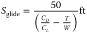
15.4.2.1 Ground Distance During Glide, Sglide
Normally, at a steady approach the aircraft is kept throttled back to idle producing no thrust. Figure 15.4 gives the generalised force diagram. It shows thrust, T, assisted by a component of weight, Wsinγ, in the descent angle, γ. In equilibrium, lift, L, is balanced by the weight component, Wcosγ. Equating for equilibrium conditions:
and D = T + W sin γ
or γ = CD/CL – T/W
Figure 15.4 gives Sglide = 50/tanγ. For a small γ, SLG = 50/γ.
Substituting the relation for γ, it gives
Velocity at touchdown = 1.15 Vstall_land.
However, as mentioned before, instead of using Eq. 15.11 the ground distance during glide, Sglide is computed as follows:
Ground distance from VB to stop, V = 0 is formulated next.
To keep the derivation generalised, negative thrust of the thrust reverser is included. However, in the Bizjet example there is no thrust reverser. (Note: the average condition is at 0.707 VTD).
where
LFL,
15.5 Climb Performance
Climb is possible when available engine thrust is more than the aircraft drag, the excess thrust (thrust minus aircraft drag, T – D, is converted into the potential energy of height gain). Figure 15.5 gives the generalised force diagram of an aircraft climb path in the wind axes in a pitch plane (vertical plane, i.e. the plane of symmetry). Here, the thrust vector is aligned to the velocity vector. Aircraft velocity is V climbing at an angle γ with an angle of attack α. To compute integrated climb performance, the climb trajectory is discretised into small steps of altitude (ΔH) within which the variables are considered invariant.
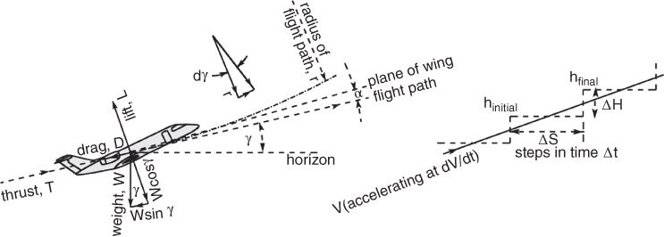
Figure 15.5 Generalised force diagram in pitch (vertical) plane – climb performance.
Note that at climb, lift, L (normal to the flight path), is lower than aircraft weight, W (vertically downward). The residual component of the weight is balanced by the excess thrust (see Eq. ). The combat aircraft or aerobatic aircraft climb angles can be high. Typically, commercial aircraft climb angle is less than 15° (cos15 = 0.96 and sin15 = 0.23). Two situations can arise as follows:
15.5.1 Derivation of Climb Performance Equations
From Figure 15.5, the force equilibrium gives (T – D) = mgsinγ + (m)dV/dt
Write dV/dt = (dV/dh) × (dh/dt), then;
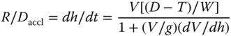
By transposing and collecting dh/dt,

For un‐accelerated rate of climb, Eq. becomes as follows.
The rate of climb is a point performance and is valid at any altitude. The term ![]() is a dimensionless term. It penalises unaccelerated rate (numerator of Eq. (15.20)) of climb depending on how fast the aircraft is accelerating during the climb. Part of the propulsive energy is consumed for speed gain instead of altitude gain. Military aircraft make an accelerated climb in the operational arena when the
is a dimensionless term. It penalises unaccelerated rate (numerator of Eq. (15.20)) of climb depending on how fast the aircraft is accelerating during the climb. Part of the propulsive energy is consumed for speed gain instead of altitude gain. Military aircraft make an accelerated climb in the operational arena when the ![]() term reduces the rate of climb depending on how fast the aircraft is accelerating. On the other hand, a civil aircraft has no demand for high accelerated climb, instead it makes en route climbs to cruise altitude at a quasi‐steady state climb by holding aircraft climb speed at a constant EAS/Mach number (very slow rate of speed change as altitude increases). Constant EAS climb makes TAS increase with altitude gain, that is, also the Mach number. A constant indication of speed eases pilot workload. During a quasi‐steady state climb at constant EAS, the contribution by the
term reduces the rate of climb depending on how fast the aircraft is accelerating. On the other hand, a civil aircraft has no demand for high accelerated climb, instead it makes en route climbs to cruise altitude at a quasi‐steady state climb by holding aircraft climb speed at a constant EAS/Mach number (very slow rate of speed change as altitude increases). Constant EAS climb makes TAS increase with altitude gain, that is, also the Mach number. A constant indication of speed eases pilot workload. During a quasi‐steady state climb at constant EAS, the contribution by the ![]() term is low. The magnitude of the acceleration term reduces with altitude gain and becomes close to zero at the ceiling (defined when R/Caccl = 100 ft min−1). (Remember: V = VEAS/√σ and VEAS = Ma√i].
term is low. The magnitude of the acceleration term reduces with altitude gain and becomes close to zero at the ceiling (defined when R/Caccl = 100 ft min−1). (Remember: V = VEAS/√σ and VEAS = Ma√i].
15.5.2 Quasi‐Steady State Climb
Civil aircraft en route climb is executed at a constant EAS when the acceleration term, ![]() ≈ 0, and dγ/dt =
≈ 0, and dγ/dt = ![]() ≈ 0. This makes the
≈ 0. This makes the ![]() term in Eq. (15.20) small enough as derived follows.
term in Eq. (15.20) small enough as derived follows.
(The other possibility is to have quasi‐level flight. This is when the climb angle, γ, is small (typically <10°) but the acceleration term, ![]() is not. sinγ ≈ γ radians, cosγ ≈ 1. It gives γ2 < < 1. This is not dealt with in this book.)
is not. sinγ ≈ γ radians, cosγ ≈ 1. It gives γ2 < < 1. This is not dealt with in this book.)
15.5.2.1 Constant EAS Climb
The term ![]() can be worked out in terms of constant EAS as follows.
can be worked out in terms of constant EAS as follows.

Below the troposphere (for air, γ = 1.4, R = 287 J kg K−1, g = 9.81 m s−2)
In SI, Eq. (1.7a) gives in troposphere T = (288.16–0.0065 h) and

Substituting the values 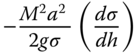 of Eq. (15.21)


Above the tropopause (for air, γ = 1.4, R = 287 J kg K−1, g = 9.81 m s−2, a = 295.07 m s−1).
From 11 to 20 km the ambient temperature is held constant at 216.65 K. Eq. (1.8g) gives the density relation in this regime as ρ kg m−3 = ![]() where base pressure ρ1 = is at 11 km.
where base pressure ρ1 = is at 11 km.
That gives σ = ρ/ρ0 = (ρ/ρ1)(ρ1/ρ0) = (ρ/ρ1)(0.36392/1.225) = 0.297 × (ρ/ρ1) = ![]()
or σ = ![]() = 0.297 × e−[0.0001578](h − 11, 000) = 0.297 × e(1.7355 − 0.0001578h)
= 0.297 × e−[0.0001578](h − 11, 000) = 0.297 × e(1.7355 − 0.0001578h)
Then (dσ/dh) = 0.297 × e(1.7355 − 0.0001578h)[−0.0001578]
Then Eq. can be written as follows.

15.5.2.2 Constant Mach Climb
The term ![]() can be worked out in terms of a constant Mach number climb as follows.
can be worked out in terms of a constant Mach number climb as follows.

![]()
Below the tropopause (for air, γ = 1.4, R = 287 J kg K−1, g = 9.81 m s−2)
From Eq. (1.7a), atmospheric temperature, T, can be expressed in terms of altitude, h, as follows:
T = (288–0.0065 h) where h is in metres. Substituting the values of γ, R and g, the following is obtained.
Substituting the value in Eq. , 

Above the tropopause (for air, γ = 1.4, R = 287 J kg K−1, g = 9.81 m s−2, a = 295.07 m s−1)
In the similar manner, the relations above the tropopause can be obtained. Above the tropopause up to 25 km, the atmospheric temperature remains constant at 216.65 K, therefore the speed of sound remains invariant, that is (da/dh) = 0 making ![]() = 0.
= 0.
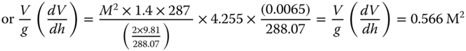
Table 15.7 summarises the relation between ![]() and the constant speed climb schedules as derived before.
and the constant speed climb schedules as derived before.
Table 15.7 The ![]() value (dimensionless quantity) at constant climb speeds (quasi‐steady climb).
value (dimensionless quantity) at constant climb speeds (quasi‐steady climb).
| Below tropopause | Above tropopause | |
| At constant EAS | 0.566 M2 | 0.7 M2 |
| At constant Mach number | −0.133 M2 | 0 (Mach held constant) |
To prepare the Pilot Manual, the airspeed needs to be in VCAS and the conversion from VEAS requires incorporating relevant errors associated with the airspeed indicator (see Section ). Readers may refer to [1] for details on compressibility correction. Nowadays, ready data is available in the Electronic Flight Information System (EFIS) memory.
With the loss of one engine at the second segment climb, an accelerated climb would penalise the rate of climb. Therefore, second segment climb with one engine inoperative is done at an unaccelerated climb speed, at a speed V2 with the undercarriage retracted. The unaccelerated climb equation is obtained by dropping the acceleration term in Eq. 15.18, yielding the following equations.
The en route climb performance parameters vary with altitude. En route climb performance up to cruise altitude is computed at discrete steps of altitude (say in steps of 5000 ft altitude – see Figure 15.5) within which all parameters are considered invariant and taken as average value within the step altitudes. The engineering approach is to compute the integrated distance covered, time taken and fuel consumed to reach the cruise altitude in steps of small altitudes and then summed up. The procedure is shown next.
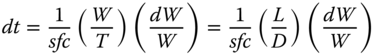
Infinitesimal time to climb is expressed as dt = dh/(R/Caccl). The integrated performance within the small steps of altitudes can be written as
The distance covered during climb can be expressed as
where V = average aircraft speed within the step altitude
Fuel consumed during climb can be expressed as
Military combat aircraft with high (TD) climb is performed in an accelerated climb. The equation for accelerated climb can be derived as follows (Figure 15.5). To keep it simpler, the subscript ∞ is dropped to represent aircraft velocity. This is not dealt with in this book.
- Summary
- Distance covered during climb, Rclimb = ∑Δs is obtained by summing up the values obtained in the small steps of altitude gain.
- Fuel to climb, Fuelclimb = ∑Δfuel is obtained by summing up the values obtained in the small steps of altitude gain.
- Time to climb, timeclimb = ∑Δt is obtained by summing up the values obtained in the small steps of altitude gain.
15.6 Descent Performance
Figure 15.6 shows the aircraft descent force and velocity diagram.
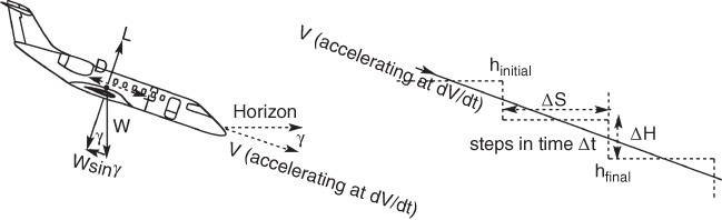
Figure 15.6 Aircraft descent force and velocity diagram.
15.6.1 Derivation of Descent Performance Equations
Descent uses the same equations, except that the thrust is less drag the rate of descent (R/Daccl) is opposite to the rate of climb. The rate of descent is expressed as follows:
Unlike climb, gravity assists descent, hence it can be performed without any thrust (engine kept at idle rating producing zero thrust). However, passenger comfort and aircraft structural considerations require a controlled descent with maximum rate limited to a certain value depending on the design as explained in Section 15.2.3. Controlled descent is carried out at a part throttle setting. To obtain maximum range, the aircraft should ideally make its descent at the minimum rate. These adjustments will entail varying speed at each altitude. To ease pilot load, descent is made at a constant Mach number and when it has reached the VEAS limit it adopts a constant VEAS descent, in a quasi‐steady state, as is done for climb. During quasi‐steady state descent at constant EAS, the contribution by the ![]() term is low.
term is low.
Some special situations may be pointed out as follows.
For unaccelerated descent Eq. gives
At a higher altitude, the prescribed speed schedule for descent is at a constant Mach, hence above the tropopause VTAS is constant and descent is kept in unaccelerated flight.
At zero thrust, Eq. 15.32 becomes
It indicates that at constant V(L/D) the R/Cdescent is the same for all weights.
As in climb, the other parameters of interest during descent are range covered (Rdescent), fuel consumed (Fueldescent) and time taken (timedescent) during descent. There are no FAR requirements for the descent schedule. Descent rate is limited by the cabin pressurisation schedule for passenger comfort. FAR requirements are enforced during approach and landing.
The descent velocity schedule is supplied to cater for the ECS capability (cabin descent rate = 300 ft min−1, actual aircraft descent is higher than that, as explained in Section 15.2.3). This requires a shallow descent gradient, part throttle is required to maintain the gradient with the benefit of distance gained during descent.
Section 15.6 gives the worked example of the Bizjet. Integrated performances for climb to cruise altitude and the descent to sea level are computed and the values for distance covered, time taken and fuel consumed are estimated to obtain the aircraft payload‐range. Reference [1] be consulted for details of climb and descent performances on this Bizjet example.
15.7 Checking of the Initial Maximum Cruise Speed Capability
At the conceptual design phase (Phase I), the aircraft sizing and engine matching exercise promised the capability to meet the customer requirement of initial maximum cruise speed and needs to be guaranteed through flight test substantiation.
Civil aircraft maximum speed is executed in an HSC in a steady level flight when the available thrust equals the aircraft drag.
The first task is to compute drag for the flight CL at the maximum cruise speed and then check if the available thrust (at maximum cruise rating of the engine) is sufficient to achieve the required speed. In some cases the available maximum cruise thrust is more than what is required; in that case the engine is adjusted to a slightly lower level. Section gives the worked‐out example.
The long range cruise (LRC) schedule is meant to maximise range and is operated at a lower speed to avoid compressibility drag rise.
15.8 Payload‐Range Capability – Derivation of Range Equations
Finally, the civil aircraft must be able to meet the payload‐range capability as specified by the market (customer) requirement. The mission range and fuel consumed during the mission are given by the following two equations.
The method to compute fuel consumption, distance covered, time taken during climb and descent is discussed in Sections 15.5 and 15.6. In this section, the governing equation for cruise range (Rcruise), cruise fuel (Fuelcruise) and time taken during cruise are derived.
Let Wi = aircraft initial cruise weight (at the end of climb) and
Wf = aircraft final cruise weight (at the end of cruise)
At any instant, rate of aircraft weight change, dW = rate of fuel burned (consumed).
In an infinitesimal time dt, the infinitesimal weight change, dW = sfc × thrust (T) × dt
In Eq. 15.37, multiply both the numerator and denominator by weight, Wand then equate T = D and W = L.
The Eq. 15.37 reduces to
Therefore, range covered during cruise (Rcruise) is the integration of Eq. 15.39 from the initial cruise weight to the final cruise weight. At cruise, V and sfc remain nearly constant. Taking mid‐cruise L/D, the change in L/D can ignored. These can be taken out of the integral sign. Eq. 15.38 gives the time taken for the Rcruise. At cruise T = D and L = W.

The value of ln(Wi/Wif) = k1_range varies from 0.2 to 0.5, longer the range, the higher the value.
Of the Eq. 15.40, the terms Wi and Wf are concerned with fuel consumed during cruise and the term sfc stems from the matched engine characteristics. The rest of the terms (VL/D) are concerned with aircraft aerodynamics. Aircraft designers aim to increase (VL/D) as best as possible to maximise range capability. The aim is not just to maximise (L/D) but to maximise (VL/D). Expressing in terms of Mach number, it becomes (ML/D). To have the best of engine‐aircraft gain it is best to maximise (ML)/(sfcD).
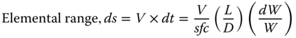
Specific range, Sp.Rn, is defined as range cover per unit weight (or mass) of fuel burned.
Using Eq. 15.40,
Cruise fuel weight (Wi − Wf) can be expressed in terms of maximum takeoff weight (MTOW) and varies from 15 to 40% of MTOW, the longer the range, the higher the value. Let k2_range = k1_range/(0.15–0.4).
Then Eq. 15.41 reduces to

Equation 15.42 gives a good insight on what can maximise range, that is, a good design to stay ahead in the competition. It says
- Make aircraft as light (MTOM) as it can be made without sacrificing safety. Material selection and structural efficiency are the keys to it. Integrate with lighter bought‐out equipment.
- Make superior aerodynamics to lower drag (high L/D).
- Choose the better aerofoil for good lift keeping the moment low.
- Make aircraft to cruise as fast it can within Mcrit (aerofoil selection).
- Match the best available engine with the lowest sfc (better engine selection).
However, Eq. 15.40 does not address the cost implications. At the end, DOC will dictate the market appeal and the designers will have to compromise performance with cost. This shows the importance of giving due consideration at the conceptual design stage to deciding on the manufacturing philosophy to be adopted to minimise aircraft production cost. These form the essence of good civil aircraft design; easily said but not so easy to achieve as must be experienced by the readers.
Equation 15.40 can be further developed. From the definition of lift coefficient, CL, the aircraft velocity, V, can be expressed as:
V = ![]() , substituting in Eq. 15.38 the cruise range Rcruise can be written as
, substituting in Eq. 15.38 the cruise range Rcruise can be written as

As mentioned earlier, typically over the cruise range, changes in sfc, and L/D are small and if the mid‐cruise values are taken as averages then they may be treated as constants and are taken out of the integral sign. Then Eq. 15.43 becomes
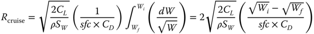
This equation is known as the Breguet Range formula, originally derived for propeller‐driven aircraft, which embedded propeller parameters (jet propulsion was not invented at that time).
LRC is carried out at the best sfc and at the maximum value of √CL/CD (i.e. L/D) to maximise range. Typically, the best L/D occurs at the mid‐cruise condition. For every LRC (say around and over 2500 nm), the aircraft weight difference from initial to final cruise is large. There is a benefit if cruise is carried out at higher altitude when the aircraft becomes lighter. This can be done either in stepped altitudes or by making a gradual shallow climb matching with the gradual lightening of the aircraft.
Sometimes, a mission may demand HSC to save time, in which case Eq. 15.44 is still valid but not operating for the best range. There are many other possibilities on how cruise segments can be executed depending on the sortie requirement as shown in [1].
15.9 In Horizontal Plane (Yaw Plane) – Sustained Coordinated Turn
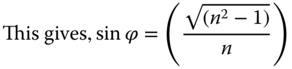
Turning is a pilot induced manoeuvre. A distinction should be made between a sustained turn in a steady state and an instantaneous turn in an unsteady state. A steady sustained turn is a coordinated turn when the load factor, n, remains constant and thrust is aligned with the velocity vector. Turning has to stay within the permissible load factor limit, nmax, (structural consideration) or within the CLstall (aerodynamic consideration) limit. Operating within these limits, an aircraft is not designed to enter into buffet. Treatment of the instantaneous turn is beyond the scope of this book – refer to [2] for the full derivation.
Forces in wind axes FW are as shown in Figure 15.7. In a coordinated turn, the roll (bank) angle is ϕ and turning angle is ψ.

Figure 15.7 Forces on an aircraft coordinated turn in the horizontal plane.
15.9.1 Kinetics of a Coordinated Turn in Steady (Equilibrium) Flight
The equation of motion at an instant of a steady turn has a radius R of turn and aircraft velocity, V, tangential to the flight path. In elemental time Δt, the turning angle is Δψ.
Then, the instantaneous angular velocity can be written as (dψ/dt) in rad s−1.
The instantaneous tangential velocity can be written as V = R(d/ψdt) in ft s−1.
The thrust line is taken along the flight path. Turn is in a bank angle of ϕ with L′ as the lift force acting at the aircraft plane of symmetry normal to the instantaneous tangential velocity V (true airspeed).
In the horizontal plane, thrust = drag
In the lateral plane, weight, W = mg = L′cosϕ
where L′ − L = ΔL = W/cosϕ – W = W(1/cosϕ − 1)
where n = aircraft load factor acting in the plane of symmetry of the aircraft along L′.
Perpendicular to a flight path towards the instantaneous centre of turn, the force balance gives:
centrifugal force = centripetal force,
Therefore, the centripetal acceleration acting radial (normal to the flight path), an = V2/R
Combining Eqs. 15.46 and 15.49,
m = L′cosϕ/g = RL′sinϕ/V2
or V2/Rg = sinϕ/cosϕ = tanϕ
Substituting Eq. 15.45,
Eq. 15.49 gives,
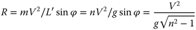
Using Eq. 15.47 n = L′/W = L′/mg, Eq. 15.54 gives the radius of turn
- Load factor, n:
From Eq. 15.53 gives, R = mV2/L′sinϕ
where, CL′ is the lift coefficient while turning under load factor, n.
where L′ = nmg = 0.5ρV2SWCL′
Substituting Eq. 15.56 into Eq. 15.55,
T = D = 0.5ρV2SW[CDPmin + k(2nmg/ρV2SW)2]
or T = 0.5ρV2SWCDPmin + k(0.5ρV2SW)(2nW/ρV2SW)2]
or T = 0.5ρV2SWCDPmin + k(2n2W2/ρV2SW)]
Solve Eq. 15.57 for load factor, n
or n2 = 
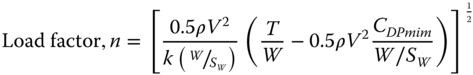
15.9.2 Maximum Conditions for a Turn in the Horizontal Plane
Differentiating Eq. 15.58 with respect to V setting it equal to zero gives the maximum conditions of Vn_max as follows.

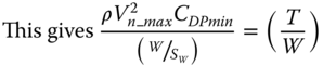
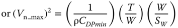
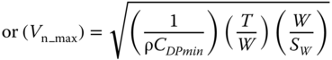
Substituting in Eq. 15.18, the maximum load factor, n, can be obtained


15.10 Aircraft Performance Substantiation – Worked‐Out Classroom Examples – Bizjet
As stated earlier that during the Conceptual Design Phase‐I, before the ‘go‐ahead’ obtained, only the specified aircraft performance requirements are to be substantiation (see Section 1.8). The specified Bizjet market requirements are given below.
- Baseline Version (8 to 10 passengers) ‐ 10 passengers at standard (medium) comfort level.
Payload: 1,100 kg
Take‐off field length (TOFL) at sea‐level STD day = 4400 ft
Landing field length (LFL) at sea‐level STD day = 4400 ft
Initial climb rate at sea‐level STD day = 2600 ft/min
Initial high speed cruise (HSC) at 41000 ft, STD day = 0.74 Mach
Range: 2,000 miles + reserve
g‐level: 3.8 to −2.
- Given below are the sized Bizjet aircraft data (see Section 14.4) for performance substantiation.
MTOM = 20 680 lb (9400 kg); wing area, SW = 323 ft2 (30 m2)
Bizjet sized wing load, W/SW = 64, TSLS/W = 0.34
At static conditions, TSLS = 3500 lb per engine, T/Wavg = 0.308
Landing weight = 15,800 lb (7182 kg)
Dynamic head, q = ½ρV2 = 0.5 × 0.002378V2 = 0.001189V2
Equations used: CL =
 =
=  =
=  , Vstall =
To make the best use of available data, all computations are done using the FPS system. The results can be subsequently converted to the SI system. Tables 15.8–15.17, present all the data required for Bizjet performance substantiation.
Table 15.8 Bizjet performance parameters (takeoff/landing – W/SW = 64 lb ft−2).
| Flap setting, deg | 0 | 8 | 20a | Landingb |
| CLmax | 1.55 | 1.67 | 1.9 | 2.2 |
| CDpmin | 0.0205 | 0.0205 | 0.0205 | 0.0205 |
| Rolling friction coefficient, μ | 0.03 | 0.03 | 0.03 | 0.03 |
| Braking friction coefficient, μB | 0.45 | 0.45 | 0.45 | 0.45 |
| Vstall @ 20 680 lb ft s−1 | 186.4 | 179.5 | 168.4 | 136.16 a |
| Vstall, knots | 110.38 | 106.00 | 99.38 | 80.66 |
| VR, ft s−1 (1.11 Vstall) | 205.08 | 196.91 | 184.61 | 149.77 |
| VR, knots | 121.5 | 116.60 | 109.32 | 88.7 |
| VLO, knots (1.15 Vstall) | 126.94 | 121.90 | 114.28 | 92.72 |
| VLO ft s−1 | 214.38 | 205.87 | 193.00 | 156.58 |
| V2, knots (1.2Vstall) | 132.46 | 127.20 | 119.25 | 96.75 |
| V2, ft s−1 (1.2Vstall) | 223.7 | 214.82 | 201.4 | 163.40 |
| T/Wavg – all‐engine | 0.308 | 0.308 | 0.308 | 0 |
| T/Wavg – single engine | 0.154 | 0.154 | 0.154 | 0 |
aNormal takeoff at STD day is carried out with a 20° flap setting. At lower takeoff weight and/or hot and high altitude airfield having longer runway length (4400 ft), the pilot may choose 8° flap that gives a better second segment climb gradient.
bLanding at 35–40° flap, engines at idle and Vstall at aircraft landing weight of 15 800 lb.
15.10.1 Checking TOFL (Bizjet) – Specification Requirement 4400 ft
During take‐off ground run, aircraft accelerates from zero to lift‐off speed, Vlift_off, causing continuous changes in aircraft aerodynamics characteristic, e.g., lift and drag. An accurate TOFL estimation requires CL and CD variation with speed gain. Readers may refer to [1] for the methodology adopted to compute accurate TOFL using a graph showing the varying force parameters during the ground run.
The acceleration term in take‐off has a strong contribution to the determination of BFL. Ref [1] shows that TOFL estimation using average acceleration gives result within 1% of the accurate TOFL value for all engine operating case. It is convenient to use average acceleration, ā, term at this stage of study.
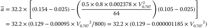
Equation gives average acceleration, ā, as follows.

The average acceleration, ā, can be applied for the segment with initial velocity, Vi, and final velocity, Vf, i.e., at 0.707V = 0.707 × (Vf − Vi) + Vi of the segment of operation
For the ground run, Eq. 15.8a gives the following.

Table 15.5 may be used for Bizjet aircraft take‐off estimation at a sea level ISA day to prepare the spreadsheet for repeated computations. Table 15.8 gives the Bizjet aircraft data generated thus far. To make the best use of the available data all computations are done in the FPS system. The results can be subsequently converted to the SI system.
At V2 speed, T@119.25 kt = 2860 lb per engine (20° flap)
Rolling friction coefficient on paved runway, μ = 0.025.
Several decision speeds are worked out to estimate takeoff capabilities. First, the all‐engine TOFL is estimated. Next, the BFL is estimated, for which the decision speed V1 is to be determined in the inadvertent case of one critical engine failure.
15.10.1.1 All‐Engine Takeoff – 20° Flap
Table 15.9 gives the values for all‐engine TOFL with the Bizjet at 20° flap. Due to extended undercarriage and flap deflection, the aircraft lift to drag ratio degrades to a typical value of approximately 10 for the Bizjet.
Table 15.9 Segment A – all‐engine operating from zero to VR (see Figure 15.1).
| Vstall | VR | |||
| V, kt | 80 | 90 | 100 | 110 |
| V, ft s−1 | 135.04 | 151.92 | 168.8 | 185.68 |
| 0.5ρSW | 0.384 | 0.384 | 0.384 | 0.384 |
| 0.707V | 95.47 | 107.41 | 119.34 | 131.28 |
| āavg | 8.91 | 8.85 | 8.793 | 8.73 |
| ΔV | 135.04 | 151.92 | 168.8 | 185.68 |
| Vavg | 67.52 | 75.96 | 84.4 | 92.84 |
| SG, ft | 1024 | 1304 | 1620 | 1976 |

15.10.1.1.1 Flare from VR to V2
The aircraft is under manoeuvre load through and in climb, and still accelerates at a lower rate. Aircraft flaring through rotation is a complex physics and is described in detail in [1]. Typically, in this class of aircraft, it takes 3 s. Here the computation is simplified by taking the average velocity from VR to V2 to cover field length distance in 3 s.
Taking flare time as 3 s for the Bizjet, the average VLO to V2 = (192.43 + 202.56)/2 = 197.496 ft s−1
Computed all‐engine operating field length = 1976 + 592.3 ≈ 2568 ft
To ensure safety, the FAR requires an all‐engine operating TOFL at a 15% higher margin than the computed value and it may exceed the value obtained for a one engine inoperative BFL value. In that case, the higher value of the two is used.
FAR all‐engine operating field length for a Bizjet at 20° flap, TOFLall_eng = 1.15 × 2568 = 2953 ft
To compare with the simplified method to compute ![]() , take average acceleration at
, take average acceleration at
![]() compared to 1976.3 ft in Table 15.9. This shows excellent agreement.
compared to 1976.3 ft in Table 15.9. This shows excellent agreement.
15.10.1.2 One Engine Inoperative – Balanced Field Takeoff (BFL) Inoperative
Section 15.3.2 gives the BFL takeoff to make sure that the aircraft can stop on the airfield in case an engine fails. It requires a decision speed V1, below which the aircraft stops and above which the aircraft continues with the takeoff operation with power available to maintain the FAR stipulated minimum climb gradient up to the second segment and then return to land immediately. At first, V1 is estimated and subsequently establishes the BFL for takeoff. Table 15.9 showing all engine takeoff values can be used up to a speed of V1.
- Segment A – all engines operating up to the decision speed V1 – BFL run
To determine the decision speed V1, estimate three speeds, for example, 80, 90 and 100 kt. The all‐engine operating case up to these speeds can be taken from Table 15.9.
- Segment B – one engine inoperative acceleration from V1 to lift‐off speed, VR
This phase is a transient one; the aircraft leaves the ground to become airborne. Its lift and drag characteristics are changing fast. With the aircraft in a high drag configuration with one engine inoperative, drag estimation is quite difficult. Therefore, a simplified approach is taken to compute distance covered and time taken from V1 to lift‐off speed, VLO. The simplification gives a reasonable result and conveys the physics involved. Industries using computers and more accurate lift and drag data adopt detailed calculations.
In flight, the lift to drag ratio in such a dirty configuration will be low, in this class in the order of around 9.5. On the ground below rotation speed, the lift is low and so is drag is low; the simplification takes the same value of (L/D) ≈ 9.5. Therefore, the average value of (CD/CL) ≈ 0.105 is taken. A typical average CL ≈ 0.8 is taken, the weight on the wheels is lighter on account of some lift generated on the wing. Because one engine is inoperative there is a loss of power by half [(T/W)avg = 0.154)]. The simplified method is used because the difference will be small.
The velocity that would give average acceleration is V0.707 = 0.7 × (VR − V1) + V1.
One engine inoperative ā for the Bizjet after decision V1 is as follows
20° flap
Braking takes place after an engine fails when it has the all‐engine acceleration. With the loss of thrust aircraft on account of engine failure the acceleration does not suddenly drop to low levels in a discrete step down, but the aircraft gradually retards to a lower level of acceleration. Therefore, for the interval of computation, the average value has to be taken. This is an important consideration that is often overlooked. āave = 0.5 × (āall_engine + āone_engine_failed)
Section gives the ground distance covered, SG = Vave × (Vf − Vi)/ā
Table 15.10 computes Segment B, the ground distance covered from V1 to VLO.
- Segment C – Flaring distance with one engine inoperative from VR to V2
Table 15.10 Segment B – the ground distance covered from V1 to VLO for the 20° flap.
| Vstall | VR | |||
| V, kt | 80 | 90 | 100 | 110 |
| V, ft s−1 | 135.04 | 151.92 | 168.8 | 185.68 |
| VLO, ft s−1 | 192.432 | 192.432 | 192.432 | 192.432 |
| ΔV | 57.392 | 40.512 | 23.632 | 6.752 |
| Vavg | 163.74 | 172.18 | 180.62 | 189.06 |
| 0.707V | 175.62 | 180.56 | 185.51 | 190.45 |
| Ā | 3.416 | 3.374 | 3.331 | 3.286 |
| āave | 6.162 | 6.114 | 6.062 | 6.006 |
| SG, ft | 1525 | 1141 | 704 | 213 |
This is the flaring distance to reach V2 from VR. From the statistics, time taken to flare is 2 s. Tables 15.10–15.12 compute the ground distance covered from VLO to V2 with one engine inoperative for the flap settings. In this segment the aircraft is airborne, hence there is no rolling friction. By taking the average velocity between V2 and VR the distance covered during flare is given.
The next step is to compute the stopping distance with the maximum application of brakes.
| Vstall | VR | VLO | V2 | |||
| V (kt) | 80 | 90 | 100 | 110 | 114 | 120 |
| Segment (B + C) | 2118 | 1734 | 1297 | 781 | 593 | 593 |
- Segment D – Engine failed (recognition time)
Table 5.12 computes the ground distance covered from V1 to VB.
Table 15.11 Segment C – Bizjet one engine ground distance VR to V2 (flaring).
| VR at 1.11Vstall f/s | 184.61 |
| VLO at 1.15Vstall f/s | 193.00 |
| V2 at 1.2Vstall f/s | 201.39 |
| Vave f/s | 197.20 |
| SGflair (3 s), ft | 591.6 |
The distance is covered in 1 s due to pilot recognition time and 2 s for the brakes to act from V1 to VB (flap settings are of little consequence).
Table 15.12 shows the Segment D engine failure recognition distance.
- Segment E – braking distance from VB to zero velocity (Flap settings are of little consequence)
Table 15.12 Bizjet failure recognition distance (Segment D).
| V – knots | 80 | 90 | 100 | 114 |
| V ft s−1 | 135.04 | 151.92 | 168.8 | 192.432 |
| Distance in 3 s at V1, SG_B – ft | 405.12 | 456 | 506.4 | 577.3 |
Reaction time to apply the brake after the decision speed, V1 is 3 s. The aircraft continues to accelerate a little in the 3 s but speed returns to VB – this is ignored. Table 15.13 computes the ground distance covered from VB to stop.
Table 15.13 Bizjet stopping distance (Segment E).
| V, kn | 80 | 90 | 100 |
| V, ft s−1 | 135.04 | 151.92 | 168.8 |
| ΔV, ft | 135.04 | 151.92 | 168.8 |
| Vavg, ft | 67.52 | 75.96 | 84.4 |
| 0.707V | 95.47 | 107.41 | 119.34 |
| Ā | −12.08 | −11.86 | −11.62 |
| SG, ft | 755 | 973 | 1197 |
| (D + E) | 1160 | 1429 | 1732 |
Aircraft in full brake mode with μB = 0.4, all engines shut down and average CL = 0.5,
Using Eq. 15.6, the average acceleration based on 0.707 VB (≈ 0.707 V1) reduces to
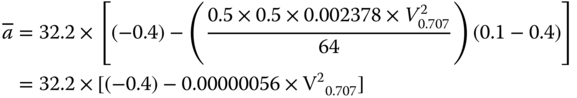
Select the distance when segments (B + C) equals segment (D + E) as shown in Figure 15.8. With 20° flap, the decision speed V1 is 94 kt covering a distance of 1570 ft. Then TOFL becomes 1430 + 1570 = 3000 ft. This is summarised in Table 15.14 and Figure 15.8. Both satisfy the specified TOFL requirement of 4400 ft.
Table 15.14 Bizjet decision speed (Figure 15.8).
| BFL | |
| Flap, degrees | 20 |
| Decision speed, V1, knots | 94 |
| Stall speed, Vstall, knots | 99.3 |
| Rotation speed, VR, knots | 109.3 |
| Lift‐off speed, VLO, knots | 114 |
| V2 speed, V2, knots | 119.3 |
| Distance, ft at (B + C) = (D + E), ft | 1570 |
| All‐engine distance at V1 speed, ft | 1430 |
| BFL, ft | 3000 |
| second segment climb gradient (computed in next chapter) | |
| All‐engine distance at V2 speed, ft | 2568 ft |
| All‐engine increase by 15% | 2953 ft |
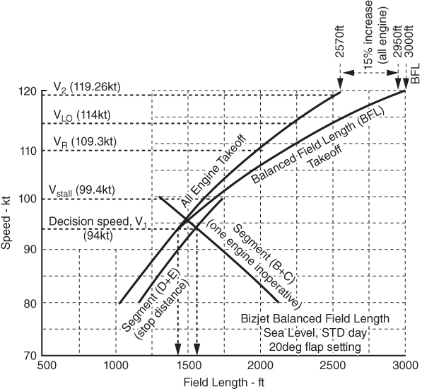
Figure 15.8 Bizjet takeoff.
The TOFL requirement is 4400 ft, recommended takeoff procedure uses a 20° flap (Figure 15.9). At lower takeoff weight and/or a longer runway length (4400 ft), the pilot may choose an 8° flap that gives a better second segment climb gradient. With the air‐conditioning switched on and at an eight flap setting, the BFL should come close to 4000 ft. The readers may compute for an 8° flap decision speed.
- Discussion for takeoff analysis
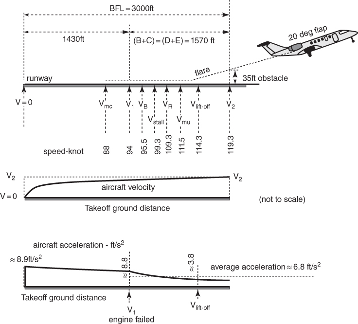
Figure 15.9 Takeoff speed schedule – 20° flap.
Increase of flap setting improves the BFL capability at the expense of a loss of climb gradient (this will be shown in the next chapter). With one engine inoperative, the percentage loss of thrust for a two engine aircraft is the highest (50% lost). With one engine failed, the aircraft acceleration suffers and the ground run taken from V1 to lift‐off is higher. Table 15.15 summarises the takeoff performance and the associated speed schedules for the two flap settings. The ratio of speed schedules can be made to vary for pilot ease, as long as it satisfies FAR requirements. This is an example of the procedure.
Table 15.15 Bizjet takeoff field length summary (Figure 15.8).
| 20 | 8 | |||
| Flap setting, degrees | knots | ft s−1 | knots | ft s−1 |
| Vstall @ 20 680 lb | 99.38 | 167.83 | 106 | 179 |
| bVmc at 0.94V1 | 84.4 b | 142.8 | 91.2 b | 153.9 |
| V1 decision speed | 90.00 | 151.92 | 96.5 | 163.74 |
| VR = 1.05Vstall | 109.32 | 184.61 | 116.60 | 196.92 |
| VLO at 1.15Vstall | 114.28 | 193.00 | 121.90 | 205.8 |
| aV2 = 1.2 Vstall at 35 ft altitude | 119.26 | 201.39 | 127.2 | 214.82 |
| Vmu at 1.02 VR (lower than VLO) | 115.50 | 188.30 | 119.00 | 200.85 |
| BFL, ft | 2940 | 3220 | ||
| All‐engine takeoff time, s | ≈31 s | |||
aIf required, V2 can be higher than 1.2 Vstall.
bAircraft control surfaces (mainly rudder) are sized to get a Vmc below V1 for the pilot to have the speed margin. Here, it arbitrarily chosen to at 75 kt – this needs to be computed (a design task beyond the scope of this book). This is because the lowest V1 is when the aircraft is lightest (say at the landing weight of 15 800 lb) and at the highest flap deployment (for an inadvertent case, it can be at 40° flap, otherwise at 20° flap). This point is often overlooked in aircraft design coursework. Figure 15.9 gives the Bizjet takeoff speed schedules.
Higher flap settings would give more time between decision speed V1 and the rotation speed VR. However, it is not a problem if V1 is close to VR, so long there is pilot reaction time is available if one engine fails; if not then in a very short time the rotation speed VR is reached and the aircraft takes off (typically, BFL is considerably less than the available airfield length). Also Vmu is close to VR, hence there is little chance for tail dragging. If the pilot makes an early rotation then Vmu may not be sufficient for a lift‐off and the aircraft will tail drag until it gains sufficient speed for the lift‐off. If the engine fails early enough then the pilot has sufficient time to recognise it and act to abort takeoff.
With more than two engines, the decision speed V1 is further away from the rotation speed VR. The pilot must remain alert as the aircraft speed approaches the decision speed V1 and must react quickly if an engine fails.
The readers should compute for other weights to prepare graphs for ISA day and ISA + 20 °C.
15.10.2 Checking Landing Field Length (Bizjet) – Specification Requirement 4400 ft
Landing weight of the Bizjet is 15 800 lb (wing loading = 48.92 lb ft−2) and at full flap 40° extended CLmax = 2.2.

Average velocity from 50 ft height to touch down = 168 ft s−1.
Distance covered before brake application after 5 s (may differ) from 50 ft height,
Aircraft in full brake with μB = 0.4, all engines shut down and average CL = 0.4, CD/CL = 0.11.
Section 15.10.1 for average acceleration based on 0.707 VTD = 110.6 ft s−1.
Then q = 0.5 × 0.002378 × 110.62 = 14.54
The deceleration equation becomes, ![]()
Deceleration, ā = 32.2 × [(−0.4) + (0.119) × (0.29)] = −11.8 ft s−2
Distance covered during braking, SG_0Land = (158 × 79)/11.8 = 1058 ft
Landing distance SG_Land = 840 + 1058 = 1898 ft
Multiplying by 1.667 (dry runway), the rated LFL = 1.667 × 1898 = 3164 ft, within requirement of 4400 ft. Typically, BFL and LFL are close to one another.
Designers must also check the capability of go‐around in case missed approach (approach climb) or baulked landing (landing climb) as described in Section 15.4.1. These cases are not worked out in this book. Generally, airfield is sufficiently long and with robust design ensures that this situation can handled by pilots. Safety can never be compromised.
15.10.3 Checking Takeoff Climb Performance Requirements (Bizjet)
There are three requirements to be substantiated for the climb performance. The three requirements are given here for the two‐engine aircraft. The first two are the FAR requirements. Table 5.3 gives aircraft configuration and FAR requirements for the first and second segment climb. The four takeoff climb segments are shown in Figure 15.3.
- Check that the FAR first segment climb requirement of positive gradient is maintained.
- Check that the FAR second segment climb gradient requirement exceeds 2.4%.
- Check the market specification of the initial en route climb rate equals or exceeds 2600 ft min−1. The cabin pressurisation system should cope with the rate of climb. This is a customer specification and not a FAR requirement.
The second segment starts at 35 ft altitude with flaps extended and undercarriage retracted (one engine inoperative) and ends at 400 ft altitude. Aircraft is maintained at V2 speed to keep the best gradient. A loss of 50% thrust does not favour accelerated climb, which will be low in the case. Engine is at takeoff rating. The available one engine installed thrust is taken from Figure 13.11. The thrust is kept invariant at takeoff rating through first segment and second segment climb. Table 15.16 summarises the first and second segment climbs for both 8° and 20° flap settings.
Table 15.16 First and second segment climb performance. Aircraft flap and undercarriage extended, engine at takeoff rating (one engine inoperative). (Use drag polar in Figures 11.2 and 11.12 to obtain drag.).
| First segment climb | Second segment climb | |||
| Up to 35 ft altitude | 35 ft to 400 ft altitude | |||
| ρave = 0.002 378 lb ft−3 | ρave = 0.002 35 lb ft−3 | |||
| 0.5ρSW = 0.379 5 | 0.5ρSW = 0.374 7 | |||
| Flap, degress | 8 | 20 | 8 | 20 |
| MTOM, kg | 20 680 | 20 680 | 20 680 | 20 680 |
| Vstall, ft s−1 (kt) | 179.6 (106.4) | 168.4 (99.8) | 179.6 (106.4) | 168.4 (99.8) |
| V2 = ft s−1 (Mach) | 216.5 (0.194) | 202.08 (0.181) | 216.5 (0.194) | 202.08 (0.181) |
| qSW = | 17 788 | 15 497.4 | 17 563 | 15 301.4 |
| CL | 1.16 | 1.33 | 1.177 | 1.35 |
| CDclean (Figure 9.2) | 0.075 | 0.1 | 0.076 | 0.101 |
| ΔCD_one_eng | 0.003 | 0.003 | 0.003 | 0.003 |
| ΔCDflap | 0.013 | 0.032 | 0.013 | 0.032 |
| ΔCD_u/c | 0.022 | 0.022 | – | – |
| CD1st_seg | 0.113 | 0.157 | 0.092 | 0.135 |
| Drag, lb | 2010 | 2433 | 1616 | 2081 |
| Thrust available, lb | 2800 | 2850 | 2790 | 2840 |
| Gradient, % | +ve | +ve | 5.4 | 3.24 |
| FAR | Meets | Meets | Meets | Meets |
15.10.4 Checking Initial En Route Rate of Climb – Specification Requirement is 2600 ft min−1
Initial en route climb starts at 1000 ft altitude (ρ = 0.0023 slug ft−3, σ = 0.9672), all engines throttled back to maximum climb rating and the aircraft has a clean configuration. The aircraft makes an accelerated climb from V2 to reach 250 KEAS, which is kept constant in a quasi‐steady state climb until it reaches Mach 0.7 at about 32 000 ft altitude, from where the Mach number is held constant in the continued quasi‐steady state climb until it reaches the cruise altitude. Fuel consumed during second segment climb is small and taken empirically (from statistics) to be 80 lb (see Table 15.17). Therefore, aircraft weight at the beginning of en route climb, W = 20 600 lb.
Table 15.17 Bizjet range (step‐climb).
| Aircraft, min | Distance, nm | Fuel, lb | Time, min | |
| weight, lb | (at end of segment) | |||
| Start and taxi out | 20 680 | 0 | 80a | 3 a |
| Takeoff to 1500 ft | 20 600 | 0 | 120 a | 5 a |
| Climb to 43 000 ft | 20 480 | 170 | 800 | 25.5 |
| Initial cruise at 43 000 ftb | 19 680 | 670 | 1460 | 100.5 |
| Initial cruise at 45 000 ftc | 18 220 | 1000 | 2000 | 150 |
| Start descent at 45 000 ft c | 16 220 | 160 | 340 | 30 |
| Approach and land from 1500 ft | 15 880 | 0 | 80 a | 5 a |
| Taxi‐in from landing weight (from reserve)d | 15 800 | 0 | 20 a | 3 a |
| Stage Total | 2000 | 4800 | 322 (5.4 h) | |
aFrom operational statistics.
bAverage specific range at 43 000 ft altitude = 0.465 nam lb−1 at average weight of ≈19 000 lb.
cAverage specific range at 45 000 ft altitude = 0.515 nam lb−1 at average weight of ≈17 000 lb.
dReserve is quite in excess of what is required. In other words, the aircraft can have a little more extra range.
At 250 kt (422 ft s−1, Mach 0.35) the aircraft lift coefficient CL = M/qSW = 20 600/(0.5 × 0.0023 × 4222 × 323)= 20 600/66150 = 0.311.
Clean aircraft drag coefficient from Figure 11.2 at CL = 0.311 gives CDclean = 0.0242.
Clean aircraft drag, D = 0.0242 × (0.5 × 0.0023 × 4222 × 323) = 0.0242 × 66 150 = 1600 lb
Available all‐engine installed thrust at maximum climb rating from Figure 13.12 at Mach 0.378 is T = 2 × 2450 = 4900 lb
From Eq. 15.20a, quasi‐steady state rate of climb is given by,
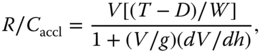
At quasi‐steady state climb, Table 15.7 gives ![]()

The capability satisfies the market requirement of 2600 ft min−1 (15.2 m s−1).
(Civil aircraft rate of climb is limited by the cabin pressurisation schedule. The aircraft is limited to 2600 ft min−1 at an altitude where the cabin pressurisation rate reaches its maximum capability. Naturally, at a low altitude of 1000 ft, this limit is not applicable.)

Figure 15.10 Climb point performances. (a) Climb speed schedule and (b) rate of climb.
15.10.5 Integrated Climb Performance (Bizjet)
Integrated climb performance is not a specification for substantiation – it is used to obtain aircraft payload‐range capability, which is a requirement to be substantiated. It is reasoned in Section 15.1 that only the results of the integrated climb performances in graphical form are given as shown in Figures 15.10 and 15.11.
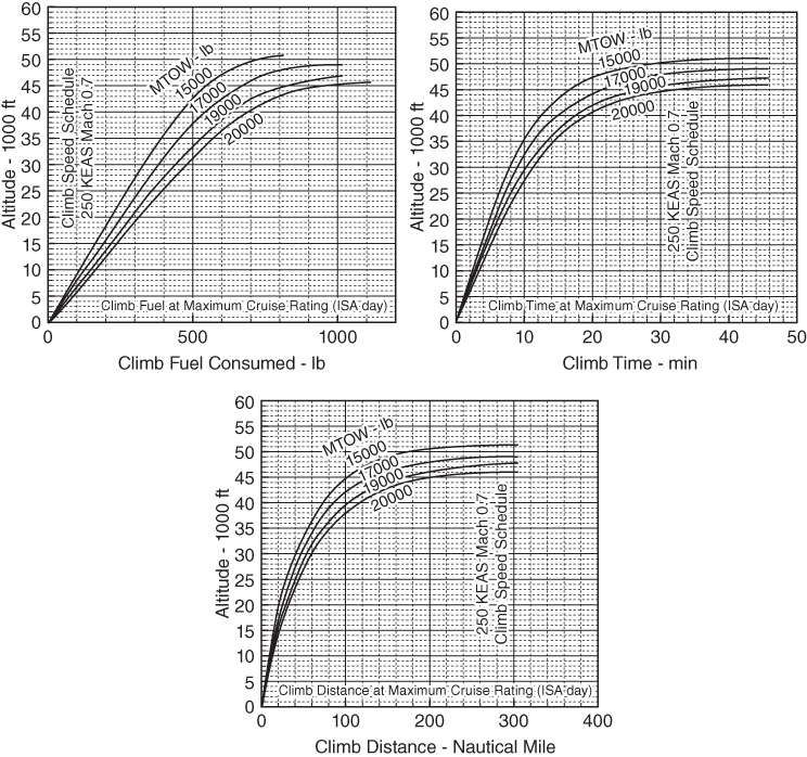
Figure 15.11 Integrated climb performances for the Bizjet (classroom example).
It is convenient to first establish the climb velocity schedule (Figure 15.10a) and the point performances of rate of climb (Figure 15.10b) up to ceiling altitudes and for at least three weights for interpolation. Bizjet carries out quasi‐steady state climb at a constant VEAS = 250 kt until it reaches Mach 0.7 and thereafter continues at constant Mach until it reaches the ceiling (rate of climb = 100 ft min−1).
The computations for the integrated climb performance are carried out in steps of approximately 5000 ft altitude (as convenient – at higher altitudes in smaller steps) in which the variables are kept invariant using their mean values (see Figure 15.5). Eqs. 15.27–15.29 are used to compute the integrated performances. Figure 15.11 gives the integrated performances of fuel consumed, distance covered and time taken to climb at the desired altitude.
The detailed computations to obtain all the graphs given in this section are shown in the companion book [1]. Classroom instructors may assist the computational work to obtain similar performance graphs for their projects.
15.10.6 Checking Initial High‐Speed Cruise (Bizjet) – Specification Requirement of High‐Speed Cruise Mach 0.75 at 41 000 ft Altitude
Aircraft at high speed initial cruise is at Mach 0.75 (716.4 ft s−1) at 41 000 ft altitude (ρ = 0.00055 slug ft−3). Fuel burned to climb is computed (not shown) to be 700 lb. Aircraft weight at initial cruise is 20 000 lb.
At Mach 0.75 the aircraft lift coefficient, CL = MTOM/qSW = 20 000/(0.5 × 0.00055 × 716.42 × 323) = 20 000/45627 = 0.438.
Clean aircraft drag coefficient from Figure 11.2 at CL = 0.438 gives CDclean = 0.0305.
Clean aircraft drag, D = 0.0305 × (0.5 × 0.00055 × 716.42 × 323) = 0.0305 × 45 627 = 1392 lb.
Available all‐engine installed thrust at the maximum cruise rating at the speed and altitude from Figure 13.13 at Mach 0.75 is T = 2 × 750 = 1500 lb (adequate).
The capability satisfies the market requirement of Mach 0.75 at HSC.
15.10.7 Specific Range (Bizjet)
Specific range is a convenient way to present cruise performance. Using Eq. 15.42 the specific range, Sp.Rn is computed. It is needed to compute the cruise segment performances (fuel, distance and time). Figure 15.12 gives the specific range for the Bizjet (classroom example).

Figure 15.12 Specific range of the Bizjet (classroom example). (a) SR at 41 000 ft altitude and (b) SR at 45 000 ft altitude.
Cruise segment distance cover is follows.
Cruise range = 2000 − (Distance to climb to 43 000 ft) − (distance to descend from 45 000 ft altitude).
From the Sp.Rn values the distance covered is worked out, which in turn gives the time taken for the distance.
15.10.8 Descent Performance (Bizjet) – Limitation Maximum Descent Rate of 1800 ft min−1
It is also reasoned in Section 15.1 that only the results of the integrated descend performance in graphical form is supplied as shown in Figures 15.13 and 15.14. It is convenient to first establish the descent velocity schedule (Figure 15.13) and the point performances of the of descent (Figure 15.14) up to sea level (valid for all weights – the difference between the weights is ignored). While redoing the calculations by the readers, there could be small differences in the results.
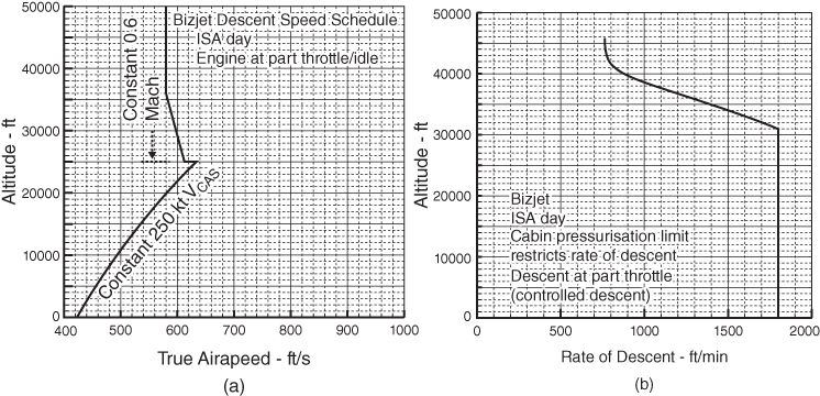
Figure 15.13 Descent point performance. (a) Descend velocity schedule and (b) rate of descent.

Figure 15.14 Integrated descent performance for the Bizjet (classroom example).
The related governing equations are explained in Section 15.6.1. It also mentions that descent rate is restricted by rate of cabin pressurisation schedule to ensure passenger comfort. Two of the difficulties in computing descent performance are to have the part throttle engine performance and the ECS pressurisation capabilities that dictate the rate of descent, which in turn stipulates the descent velocity schedule. These are not supplied in the book. Classroom instructors are to assist to establish these two graphs. In absence of any information these two may be used. The following simplifications could prove useful.
The first simplification is in obtaining part throttle engine performance as follows.
- Descent is carried out anywhere at 50–70% of maximum power rating.
- Zero thrust at idle rpm at about 40% of the maximum rated power/thrust.
The second simplification is that the descent velocity schedule is supplied to cater for the ECS capability (cabin descent rate = 300 ft min−1, actual aircraft descent is higher than that – Figure 15.13b). This is explained in Section 15.2.3.
In industry, the exact installed engine performance at each part throttle condition is computed from the engine deck supplied by the manufacturer. Also, the ECS manufacturer supplies the cabin pressurisation capability from which aircraft designers work out the velocity schedule.
The inside cabin pressurisation is restricted to an equivalent rate of 300 ft min−1 at sea level to ensure passenger comfort. The aircraft rate of descent is then limited to the pneumatic capability of the ECS. The Bizjet is restricted to a maximum of 1800 ft min−1 at any time (for higher performance, at lower altitudes it can be raised up to 2500 ft min−1). Descent speed schedule is to continue at Mach 0.6 from cruise altitude until it reaches the approach height when it changes to constant VEAS = 250 kt until the end (for higher performance, it can be raised to Mach 0.7 and VEAS = 300 kt). The longest range can be achieved at minimum rate of descent. Evidently, these will require throttle dependent descents to stay within the various limits.
It is convenient to establish first the point performances of velocity schedule (Figure 15.13a) and rate of descent (Figure 15.13b – all weights – variation is small). Descent is performed within the limits of human comfort level. However, in an emergency, rapid descent becomes necessary to compensate for loss of pressure and recover oxygen.
Integrated descent performance is computed in the same way as for climb. The integrated descent performance is computed in steps of approximately 5000 ft altitude (or as convenient) in which the variables are kept invariant. No computational work is shown here.
Figure 15.14 plots the fuel consumed, time taken and covered during descent from ceiling altitude to sea level. While redoing the integrated descent performances by the readers, there could be small differences in the results.
15.10.9 Checking out the Payload‐Range Capability – Requirement of 2000 nm
A typical transport aircraft mission profile is shown Figure 15.15.
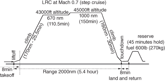
Figure 15.15 Bizjet mission profile.
Equations 15.34–15.35 give the mission range and fuel consumption expressions as:
where Rclimb = ∑Δsclimb and Rdescent = ∑Δsdescent computed from steps of heights.
where Fuelclimb = ∑Δfuelclimb and Fueldescent = ∑Δfueldescent computed from steps of heights.
Minimum reserve fuel is computed for an aircraft holding an 5000 ft altitude at around Mach 0.35–0.4 at about 50% of the maximum rating for 45 min or an 100 nm diversion cruising at 0.5 Mach and 25 000 ft altitude plus 20 min. The amount of reserve fuel has to be decided by the operator suited to the region of operation. The worked‐out example takes the first option.
Fuel is consumed during taxiing, takeoff and landing without any range contrition and this fuel is to be added to the mission fuel with the total, known as block fuel. The time taken from the start of the engine at the beginning of the mission to the stop of the engine at the end of the mission is known as block time, in which a small part of time is not contributing to gain in range. Taken from the statistics of operation, these additional fuel burn and time consumed without contributing to range are given in Table 15.17.
Reserve fuel: At 5000 ft altitude (ρ = 0.00204 lb ft−3) and 0.35 Mach (384 ft s−1) it gives CL = 0.323 resulting in CD = 0.025 (Figure 9.2). Equating thrust to drag, T/engine = 610 lb. Corresponding fuel flow rate at this speed altitude is 210 lb/h per engine; holding for 45 min consumes 2 × 0.75 × 210 = 315 lb. It is safer to keep more in reserve if a 100 nm diversion is required, which is not a stipulation if 45 min hold is taken. Therefore, it is decided to carry 600 lb reserve fuel for holding/diversion around landing airfield. The range performance can be improved with a step‐climb from 43 000 to 45 000 ft as the aircraft becomes lighter with fuel consumed.
The cruise altitude of the Bizjet starts at 43 000 ft and ends at 45 000 ft (the design range is long to make a step cruise). Taking the average value of cruising at 44 000 ft (ρ = 0.00048 slug ft−3), The methods to compute Rclimb and Rdescent are discussed in Sections 15.5 and 15.6. Using Figures 15.11 and 15.14, the required values are given as Rclimb = 170 nm, Fuelclimb = 800 lb, Timeclimb = 25 minutes, Rdescent = 160 nm and Fueldescent = 340 lb and Timedescent = 30 minutes (in part throttle gliding descent). Table 15.17 gives the segment details of aircraft weight, distant covered, fuel burned and time taken. The aircraft is at LRC schedule operating at Mach 0.7.
Table 15.17 gives the following.
MTOM = 20 680 lb (9400 kg)
Landing weight = 20 680–5500 (onboard fuel) + 600 (reserve fuel, not consumed) = 15 780 lb (rounded to 15 800 lb).
Initial and final cruise weights can then be computed from the climb and descent performance data (Figures 15.11 and 15.14, respectively) = 800 lb and 340 lb, respectively.
Initial cruise weight Wicr = 20 680 (MTOM) + 80 (taxi) + 340 (takeoff) − 800 (climb) = 19 680 lb
Final cruise weight Wfcr = 15 800 (landing weight) + 340 (descent) + 80 (taxi‐in) = 16 220 lb
Available cruise fuel = 19 680–16 220 = 3460.
Split the fuel load to 1460 lb cruising at 43 000 ft altitude and climb to 45 000 ft to use the 2000 lb fuel.
In operational practice, it is not done in this way. This example is to demonstrate the capability and logic of the operation. It can be seen that the step‐climb part has not been computed. It assumes that it is a discrete jump without losing fidelity to get the extent of possible range. Industries meticulously plan stage to make the climb to get the best range. Today, microprocessor‐based FBW operation makes the optimised cruise operation that is in a continuous shallow climb. Aircraft Performance Management (APM – see Section 16.5.2) is integral to flight and fleet management. There are several ways to climb, cruise and descend, treated extensively in Ref. [1].
In case, the specific range graphs are not available, the cruise segment range can also be obtained as shown next. First, compute the thrust required. Then from the sfc of the engine the fuel flow rate can be obtained and using the time required for the sector length, fuel required is computed.
From Table 15.17, the mid‐cruise weight is (19 700 + 16 240)/2 = 17 970 lb.
LRC is at Mach 0.7 (677.7 ft s−1, 401.5 kt). Engine power setting is below maximum cruise rating.
Aircraft lift coefficient, CL = 17 970/(0.5 × 0.00046 × 677.72 × 323) = 17 970/34120 = 0.527.
From Figure 11.2 the clean aircraft drag coefficient, CD = 0.033.
Aircraft drag, D = 0.033 × (0.5 × 0.00046 × 677.72 × 323) = 0.033 × 34 120 = 1126 lb.
Thrust required per engine is 1126/2 = 563 lb. Figure 13.13 is meant for maximum cruise rating to achieve HSC. Therefore, at LRC at Mach 0.7 it is throttled back with reduced fuel flow, sfc stays the same. From Figure 13.4, the sfc at the speed and altitude is 0.72 lb h−1 lb−1 Fuel flow for two engines = 0.72 × 1126 = 811 lb h−1 at 43 000 ft.
Mission range satisfies the requirement of 2000 nm. Block time for the mission is 5.45 h and block fuel consumed is 4923 lb (2233 kg). On landing, the return taxi‐in fuel of 20 lb is taken from the reserve fuel of 600 lb (45 min holding or diversion). Total onboard fuel carried is therefore: 4880 + 600 = 5480 ≈ 5500 lb (2500 kg).
This checks the Bizjet weights breakdown given in Table 15.17.
The payload‐range graph is given in Figure 15.16. A summarised discussion of the Bizjet design is given in Section 15.13.1.
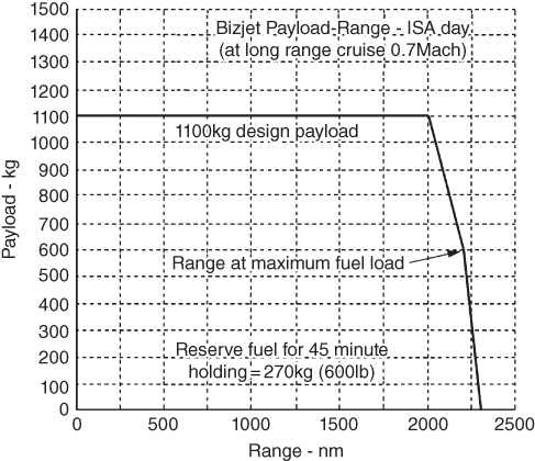
Figure 15.16 Bizjet payload‐range capability.
The fuel tank has a larger capacity than what is required for the design payload‐range. Payload could be traded to increase range until the tanks fill up by trading the payload. Further reduction of payload would make the aircraft lighter, thereby increasing the range.
15.11 Aircraft Performance Substantiation – Military AJT
Military aircraft certification standards are different from civil aircraft certification standards. There is one for customer specifications and the design standards vary from country to country based on their defence requirements. In allied international collaborative projects the customers are only the participating countries, export potential is the fall‐out of the project. The certification requirement issues have a similarity in their reasoning but differ in the requirements. Readers are suggested to obtain the regulatory military requirements from their respective Ministry/Department of Defence – these are generally available in public domain. In this book, the substantiation procedure is the same as for the civil aircraft case covered in detail in the previous section.
h3
15.11.1.1. AJT data
- AJT Requirement Specifications
Payload: 1,800 kg
Take‐off field length (TOFL) at sea‐level STD day = 3600 ft (1,100 m)
Landing field length (LFL) at sea‐level STD day = 3600 ft (1,100 m)
Initial un‐accelerated climb rate at sea‐level STD day = 10000 ft/min
Initial high speed cruise (HSC) at 30000 ft, STD day = Mach 0.85
Radius of action = 400 km + reserve
g‐level: 7 to −3.5.
| NTCMa = 4800 kg (10 800 lb) | Wing area = 17 m2 (183 ft2) |
| MTOM = 6500 kg (15 210 lb) | Engine data – Figure 13.15 |
Normal Training Configuration Mass.
The computation shown here is a short‐cut one to show AJT capability. The readers may undertake the formal approach as was done for the Bizjet.
15.11.1.5. Mission Profile
Fuel load and management depends on the type of mission. Military mission profiles are varied. Figure 15.17 gives a typical normal training profile to gain airmanship and navigational skills in an advanced aircraft.
The training profile segment breakdown is given in Table 15.18.
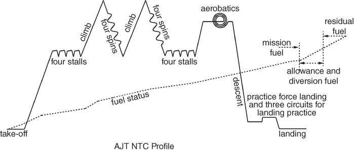
Figure 15.17 Normal training sortie profile (60 min). A – four turns and four stalls, B and C – two four turn spins, D – aerobatics, E – practise force landing.
Table 15.18 AJT engine ratings – detailed segments (fuel and time computed in Table 15.20).
| Engine rating = % rpm | |
| Taxi and takeoff | 60% (idle) |
| takeoff and climb to 6 km altitude | TO @ 100% then @ 95% |
| Four turns/stalls | 1 min @ 95% + 3 min @ 60% |
| Climb from 5 to 8 km altitude | 95% |
| Four turn spins | 60% |
| Climb from 5 to 8 km altitude | 95% |
| Four turn spins | 60% |
| Four turns/stalls | 1 min @ 95% + 3 min @ 60% |
| Climb from 5 to 6 km altitude | 95% |
| Aerobatics practise | 95% |
| Descent and practice force landing | 2 min @ 95% + 6 min @ 60% |
| Three circuits for landing practise | Average 80% |
| Approach, land return taxi | 60% |
| Trainee pilot allowance | 95% |
Block fuel and block time are computed by adding fuel and time consumed in each segment. However, distance covered is meaningless as the aircraft returns to the base. Armament training practise closely follows the combat mission profile. Combat missions depend on target range and the expected adversary defence capability. Two typical missions are shown in Figure 15.18. Air defence would require continuous intelligence information feedback.
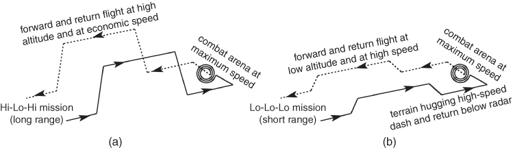
Figure 15.18 Typical combat profile. (a) A hi‐lo‐hi mission (longer distance) and (b) lo‐lo‐lo mission (shorter distance).
The study of a combat mission requires complex analysis by specialists. Defence organisations conduct these studies and are understandably kept confidential in nature. Game theory, twin dome combat simulations and suchlike are some of the tools for such analysis. Actual combat may yet prove quite different as not all is known about the adversary's tactics and capabilities. Detailed study is beyond the scope of this book and possibly of most academies.
15.11.2 Checking TOFL (AJT) – Specification Requirement 3600 ft (1100 m)
Being single engine, there is no question regarding BFL. Military aircraft TOFL must satisfy the CFL. The CFL can also have a decision speed V1, which is determined by whether the pilot can stop within the distance available, or otherwise the pilot needs to eject.
To obtain the CFL for a single engine aircraft, the decision speed is at the critical time just before the pilot initiates rotation at VR. Then the decision speed V1 is worked out from the VR by giving 1 s as the recognition time. Engine failure occurring before this V1 leads the pilot to stop the aircraft by applying full brakes and deploying any other retarding facilities available, for example a brake‐parachute. There should be sufficient runway available for the pilot to stop the aircraft from this V1. If there is not enough runway available, then a new decision speed V1, considerably lower than the VR, has to be worked out in a similar manner as done for the Bizjet. Engine failure occurring after the V1 means the pilot will have little option other than to eject (if there is not enough runway/clearway available to stop). For multi‐engine aircraft, determining the CFL follows the same procedure as the civil aircraft computation but complying with Milspecs.
In this book, the following three (CFL) requirements for the AJT are worked out.
- (i) To meet the takeoff distance of 3600 ft (1100 m) to clear 15 m
- (ii) To meet the initial rate of climb (unaccelerated): 10 000 ft min−1 (50 m s−1)
- (iii) To meet the maximum cruise speed of Mach 0.85 at 30 000 ft altitude
MIL‐C501A requires a rolling coefficient μ = 0.025 and minimum braking coefficient μB = 0.3. Training aircraft will have a good yearly utilisation operated by relatively inexperienced pilots (with about 200 h of flying experience) carrying out a very large number of take‐offs and landings on relatively shorter runways. AJT brakes are generally more robust in design giving a brake coefficient, μB = 0.45, which is much higher than the minimum Milspec requirement. Figure 15.19 gives the speed schedules of single engine military type aircraft.
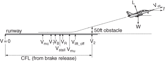
Figure 15.19 AJT takeoff.
Both the Bizjet and the AJT have the same class of aerofoil and same types of high‐lift devices. Therefore, there is a strong similarity in the wing aerodynamic characteristics. Table 15.19 gives the AJT data pertinent to takeoff performance.
Table 15.19 AJT distance, SW = 17 m2 (183 ft2).
| Flap setting – degrees | 0 | 8a | 20 a | Landing a |
| CDpmin | 0.0212 | 0.0212 | 0.0212 | 0.0212 |
| CLmax | 1.5 | 1.65 | 1.85 | 2.2 |
| ΔCDflap | 0 | 0.012 | 0.03 | 0.3 |
| ΔCD_U/C | 0.0222 | 0.022 | 0.0212 | 0.021 |
| Rolling friction coefficient, μ | 0.025 | 0.025 | 0.025 | 0.025 |
| Braking friction coefficient, μB | 0.3 | 0.3 | 0.3 | 0.3 |
| Vstall @ 10 582 lb – fts−1 | 180 | 171.7 | 162.1 | 133 |
| VR – kt (1.688 ft s−1) @ 1.11 Vstall | 112.9 (190.6) | 106.6 (180) | 87.5 (147.65) | |
| VLO – kt (1.688 fts−1) @ 1.12 Vstall | 114 (192.5) | 107.6 (181.6) | 88.3 (149) | |
| V2 – kt (1.688 ft s−1) | 122 (206) | 115.2 (194.5) | 94.5 (159.6) | |
| (T/W)avg | 0.51 | 0.51 | 0.51 | 0 |
| W/SW – lb ft−2 | 58 | 58 | 58 | 46.26 |
| CD/CL at ground run | 0.1 | 0.1 | 0.1 |
aTakeoff at 8° and 20° flaps. Landing at 35–40° flap, engines at idle and Vstall at aircraft landing weight of 8466 lb.
Equation 15.6 gives average acceleration as ā = g [(T/W – μ) – (CLSq/W)(CD/CL – μ)]
Using the values given in Table 15.19,
15.11.2.1 Takeoff with 8° Flap
Refer to Figure 15.19 showing an AJT takeoff profile.
- Distance covered from zero to the decision speed V1
The decision speed V1 is established as the speed at 1 s before the rotation speed VR. Estimate the acceleration of 16 ft s−2 (can be computed first and then iterate without estimation).
Aircraft velocity at 0.707 V1 = 122.22 ft s−1.
Up to V1, the average CL = 0.5 (still at low incidence)
Using Eq. 15.8b, the distance covered until lift‐off speed is reached,
However, provision must be made if the engine fails at the decision speed, V1, when braking has to be applied to stop the aircraft. The designers must make sure that the operating runway length is adequate to stop the aircraft.
If the engine is operating, then the AJT continues with the takeoff procedure when lift‐off takes place after rotation is executed at VR.
- Distance covered from zero to lift‐off speed VLO
Using the same equation for distance covered up to the decision speed V1 with the change to lift‐off speed, VLO = 192.5 ft s−1. Aircraft velocity at 0.707 VLO = 134.75 ft s−1.
Up to VLO, the average CL = 0.5 (still at low incidence)
Then ā = 32.2 × (0.51 − CLq/773.33) = 32.2 × (0.51–4.35/773.33) = 32.2 × 0.5004 = 16.24 ft s−2.
Using Eq. , the distance covered until lift‐off speed is reached,
- Distance covered from VLO to V2
The flaring distance is required to reach V2 clearing the 50 ft obstacle height from VLO. From statistics; the time taken to flare is 3 s with at 8° flap and at V2 = 206 ft s−1.
In 3 s the aircraft would cover SG_LO_V2 = 3 × 206 = 618 ft.
- Total takeoff distance
The takeoff length is SG_LO + SG_LO_V2 = (1140 + 618) = 1758 ft, much less than the required TOFL is 3500 ft to cater for the full weight 6800 kg (≈15 000 lb) for armament training. In that case, a higher flap setting of 20° may be required. At a higher flap setting, the aircraft will have a shorter CFL for the same weight.
- Stopping distance and the CFL
The next step is to check what is required to stop the aircraft if an engine has failed at V1. Stopping distance has three segments. CFL is normally longer than TOFL.
- Distance covered from zero to the decision speed V1, SG_1. It is computed as before to be 912 ft.
- Distance covered from V1 to braking speed VB, SG_1_B.
- Braking distance from VB (≈V1) to zero velocity, SG_B_0.
The other two are estimated here:
- Distance covered from V1 to braking speed VB
At engine failure, assume 3 s for pilot recognition and taking action. Therefore, the distance covered from V1 to VB is SG_1_B = 3 × 174.6 = 524 ft
- Braking distance from VB (≈V1) to zero velocity (flap settings are of little consequence)
The most critical moment of brake failure is at the decision speed V1 when the aircraft is still on the ground. With full brake coefficient μ = 0.45 and average CL = 0.5, V1 = 174.6 ft s−1
Aircraft velocity at 0.707 V1 = 122.22 ft s−1.
The equation for average acceleration reduces to

Using Eq. , the distance covered till lift‐off speed is reached,
Therefore, the minimum runway length (CFL) for takeoff should be = SG_1 + SG_1_B + SG_0
TOFL = 940 + 524 + 1119 = 2583 ft. It is still within the specified requirement of 3600 ft.
The takeoff length is thus 1746 ft, much less than the CFL of 2511 ft computed before. The required TOFL is 3500 ft to cater for the full weight 6800 kg (≈15 000 lb) for armament training. In that case, a higher flap setting of 20° may be required. At a higher flap setting the aircraft will have a shorter CFL for the same weight.
Evidently, the length of the runway available will dictate the decision speed V1. If the airfield length is much longer then the pilot may have a chance to set down the aircraft if an engine failure occurs immediately after lift‐off and it may be possible to stop within the available airfield length, which must have some clearway past the runway end.
Compare with the minimum Milspec requirement of breaking friction, μ = 0.3.
The equation for average acceleration reduces to
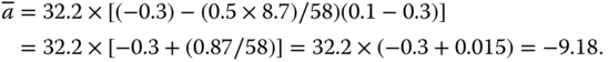
Using Eq. 18b, the distance covered from VB to zero
This value is on the high side.
The minimum runway length for takeoff should be = SG_1 + SG_1_B + SG_0
The CFL (critical field length) = 912 + 524 + 1660 = 3096 ft is on the high side but within the specification of 3600 ft. It is for this reason that a higher brake coefficient of 0.45 is taken. This is not a problem as nowadays wheels with good brakes have much a higher friction coefficient μ.
A reduction of the decision speed to 140 ft s−1 (83 kt) would reduce the SG_0 = 1068 ft bringing down the CFL to 2504 ft.
15.11.3 Checking the Second Segment Climb Gradient at 8° Flap
V2 = 206 ft s−1 (see Table 15.19) and W = 10 580 lb (4800 kg)
Clean aircraft drag coefficient from Figure 11.12 gives CDclean = 0.098.
Available thrust is 5100 lb (from Figure 13.15).
At V2 speed to clear 50 ft, the climb is at an unaccelerated rate but thereafter it will be at an accelerated rate. From Eq. steady state rate of climb is given by,
Hence, R/Caccl = {[206 × (5100–2995) × 60]/10 580} = (206 × 2005 × 60)/(10 580) = 2388 ft min−1
The capability satisfies the military requirement of 500 ft min−1 (2.54 m s−1). The reader may check for the 20° flap setting.
15.11.4 Checking Landing Field Length (AJT) – Specification Requirement 3600 ft
Keeping a reserve fuel of 440 lb (200 kg), the landing weight of the AJT is 8466 lb (wing loading = 42.26 lb ft−2) and at full flap extended CLmax = 2.2.

Vappr = 1.2Vstall@land = 160 ft s−1
VTD = 1.1Vstall@land = 146 ft s−1
Average velocity from 50 ft height to touch down = 153 ft s−1.
Distance covered before brake application after five seconds from 50 ft height,
SG_TD = 5 × 153 = 765 ft.
Aircraft in full brake with μB = 0.45, all engines shut down and average CL = 0.5, CD/CL = 0.1.
Average speed at 0.707 VTD = 107.1 ft s−1.
Then q = 0.5 × 0.002378 × 107.12 = 15.64

Distance covered during braking, SG_0Land = (146 × 73)/12.93 = 824 ft
Landing distance SG_Land = 765 + 824 = 1742 ft
Multiplying by 1.667, the rated LFL = 1.667 × 1742 = 2649 ≈ 2650 ft. It is within the specification of 3600 ft, the margin allowing for higher MTOM = 15 210 lb loaded with armament.
15.11.5 Checking the Initial Climb Performance – Requirement 50 m s−1 (10 000 ft min−1) at Normal Training Configuration (NTC)
Military trainers should climb at a much higher rate of climb than civil aircraft. The requirement of 50 m s−1 (10 000 ft min−1) at NTC is for unaccelerated climb as a capability for comparison. Unaccelerated rate of climb varies depending on the constant speed (EAS) climb, making comparison difficult. This section shows calculations for both the rates of climb.
This section will check only the en route climb with clean configuration. Unaccelerated climb Eq. is used. MTOM at NTC is 4800 kg (10 582 lb). Wing area SW = 17 m2 (183 ft2).
At en route climb, the aircraft has a clean configuration. Under maximum takeoff power, it makes an accelerated climb to 800 ft (ρ = 0.00232 slug ft−3, σ = 0.9756) from the second segment velocity of V2 to reach a 350 KEAS climb speed schedule to start the en route climb. At en route climb the engine throttle is retarded to maximum climb rating. The quasi‐steady state climb schedule holds to 350 KEAS and the aircraft accelerates with altitude gain at a rate of dV/dh until it reaches Mach 0.8 around 25 000 ft, from where the Mach number is held constant until it reaches the cruise altitude. Consider that 100 kg of fuel is consumed to taxi and climb to 800 ft altitude where the aircraft mass is 4700 kg (10 362 lb).
At 350 kt (590.8 ft s−1, Mach 0.49) the aircraft lift coefficient
Clean aircraft drag coefficient from Figure 11.17 at CL = 0.141 gives CDclean = 0.0225
Available engine installed thrust at maximum continuous rating (95% of maximum thrust given in Figure 13.15) at Mach 0.49 (459.8 ft s−1) is T = 0.95 × 5200 = 5016 lb.
From Eq. , the accelerated rate of climb as follows.
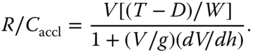
At quasi‐steady state climb, Table 15.5 gives  = 0.56 M2 = 0.56 × 0.492 = 0.1345
On substitution, rate of climb,
Therefore, an unaccelerated rate of climb, R/C = 11 395 ft min−1.
Aircraft specification is based on a constant EAS climb rate of 10 000 ft min−1, which is just met. There are many ways to climb that are dealt with in detail in [1]. (Here, the cabin area is small and the pressurised pilot suit allows a high rate of climb.)
15.11.6 Checking the Maximum Speed – Requirement Mach 0.85 at 30 000 ft Altitude at NTC
Aircraft at HSC is at Mach 0.85 (845.5 ft s−1) at 30 000 ft altitude (ρ = 0.00088 slug ft−3). Fuel burned to climb is computed (not shown) to be 582 lb. Aircraft weight at the altitude is 10 000 lb.
At Mach 0.85 the aircraft lift coefficient CL = MTOM/qSW = 10 000/(0.5 × 0.00088 × 845.52 × 183) = 10 000/57561.4 = 0.174.
Clean aircraft drag coefficient from Figure 11.17 at CL = 0.174 gives CDclean = 0.025 (high speed)
Clean aircraft drag, D = 0.025 × (0.5 × 0.00088 × 858.52 × 183) = 0.025 × 57 561.4 = 1440 lb.
Available engine installed thrust at maximum cruise rating (90% of the maximum rating) is taken from Figure 13.15 at Mach 0.85 and 30 000 ft altitude as T = 0.9 × 2000 = 1800 lb.
Therefore, the AJT satisfies the customer requirement of Mach 0.85 at HSC.
15.11.7 Compute the Fuel Requirement (AJT)
Other than ferry flight, a military aircraft is not merely dictated by the cruise sector unlike a civil aircraft mission. A short combat time at maximum engine rating, mostly at low altitudes, is a good part of fuel consumed. However, the range to the target area would dictate the fuel required. Long distance ferry flight and the combat arena will require additional fuel carried by drop tanks. Just before combat, the drop tanks (by that time they are empty) could be jettisoned to gain aircraft performance capability. The CAS variant has these types of mission profiles.
A training mission has varied engine demand and it returns to its own base covering no range as can be seen in Figure 15.20. Mission fuel is computed sector by sector of fuel burn as shown next for the classroom example. To compute fuel requirement, climb and specific range graphs for the AJT at NTC are required (Figures 15.20 and 15.21). To compute the varied engine demand of a training mission profile, use sfc and Figure 13.15 to establish the fuel flow rate for the throttle settings. The graph is valid for 75% rpm to 100% ratings. Typically, it will have approximately the following values.

Figure 15.20 AJT climb performance.
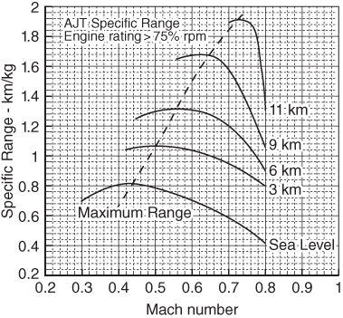
Figure 15.21 AJT specific range.
At idle (60% rpm) ≈ 8 kg min−1 At 75% rpm ≈ 11 kg min−1 At 95% rpm ≈ 16.5 kg min−1.
Fuel and time consumed for the normal training profile of the AJT is given in Table 15.20.
Table 15.20 AJT mission fuel and time consumed.
| Fuel burned, kg | Time, minutes | Engine rating = % rpm | |
| Taxi and takeoff | 60 | 6 | 60% (idle) |
| Takeoff and climb to 6 km altitude | 125 | 5 | TO @ 100% then @ 95% |
| Four turns | 50 | 4 | 1 min @ 95% + 3 min @ 60% |
| Four stalls | 60 | 5 | 1 min @ 95% + 4 min @ 60% |
| Climb from 5 to 8 km altitude | 50 | 3 | 95% |
| Four turn spins | 25 | 3 | 60% |
| Climb from 5 to 8 km altitude | 50 | 3 | 95% |
| Four turn spins | 25 | 3 | 60% |
| Climb from 5 to 6 km altitude | 15 | 1 | 95% |
| Aerobatic practise | 70 | 6 | 95% |
| Descent and practise force landing | 95 | 8 | 2 min @ 95% + 6 min @ 60% |
| Three circuits for landing practise | 110 | 10 | Average 80% |
| Approach, land return taxi | 40 | 4 | 60% |
| Trainee pilot allowance | 30 | 2 | 95% |
| Total mission fuel | 805 | 59 (≈60) | |
| Diversion | 200 | ||
| Residual fuel | 105 | ||
| Total onboard fuel | 1110 (conservative estimate) (internal fuel capacity = 1400 kg) |
15.11.8 Turn Capability – Check nmax at the Turn (AJT)
Specified g‐level: 7 to −3.5. The specification of n = 7 is the maximum permitted g‐level (nmax) in pitch plane. The specified practice tight turns has n = 4 at sea level.
Turning Eq. 15.60 gives nmax = 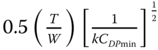 .
.
To demonstrate the AJT turn capability, let the tight turn maneuver is executed at Mach 0.5 to 0.55 at mid‐sortie weight of about 90% of NTC weight at sea level. For the AJT, Figure 14.5 gives the installed thrust loading (TSLS/W) = 0.55. Tight turning is a short duration maneuver executed that can be carried out at full throttle, but in this carried out at maximum continuous rating at 0.9 × TSLS. There operating (T/W) = (0.9 × 0.55)/(0.9 × NTC weight) ≈ 0.55.
On substitution, becomes it becomes.
nmax = 0.5 × 0.55 × √[1/(0.07 × 0.0212)] = 0.275 × √ 674 = 7.1, i.e. have excess capacity to carry out practice tight turns at around 10,000 ft altitude at n = 4.
Thrust at 10000 ft turning at a speed Mach 0.5 to 0.55 gives thrust at maximum continuous rating, T/W = 0.9 × 0.692 × (TSLS/W) = 0.623 × (TSLS/W).
On substitution, nmax at 10000 ft is as follows.
nmax = 0.5 × 0.623 × 0.55 ×√[1/(0.07 × 0.0212)] = 0.171 ×√674 = 4.43 with a healthy margin over n = 4.
Tight turning at full throttle permits n = 4 at higher altitudes.
15.12 Propeller‐Driven Aircraft – TPT (Parabolic Drag Polar)
Turboprop thrust is obtained by extracting turbine power through a propeller and therefore the related equations require additional manipulation incorporating the propeller characteristics to obtain engine power. This subsection is devoted to deriving the expressions to obtain power required by the turboprops to produce the required thrust. All derivations in this subsection are also applicable to propeller‐driven piston engine aircraft.
To develop thrust for equilibrium flight, (TP)reqd is the thrust power required from the turboprop engine. It is power [(ESHP)reqd] and not thrust force. Thrust is obtained by taking into account the propeller efficiency, ηprop (propeller characteristics), as given in Eqs. (12.35) and (12.36).
To cruise at CL at (L/D)max, turboprop aircraft equations use the terms ![]() and
and ![]() (not derived here – refer to [1]).
(not derived here – refer to [1]).
- Power required – (TP)reqd
In equilibrium level flight, power required by propeller‐driven aircraft is expressed as

Figure 15.62 is valid for both turboprop and piston engine applications. In imperial units, the turboprop is measured in shaft power (SHP) and piston engine in horsepower (HP).
Power generated by turboprop engines to produce the propeller thrust is related by Eq. (7.21) incorporating propeller efficiency ηprop as
(ESHP: Equivalent Shaft Horse Power.) At a steady level flight L = W,
where k = (1/eπAR)
For a particular aircraft, CDpmin, k and ηprop are constant, which makes this equation
where k1 = 0.5/ηprop and k2 = (k × 0.5 × ρ)/ηprop
15.13 Summarised Discussion of the Design
This is the culminating chapter of the progress made thus far on configuring, sizing and substantiation of classroom examples. It is a good time to review the designs of the Bizjet and the AJT, should they need any revision. Having commonality in design considerations, turboprop aircraft computations are not taken up here. The rest of the book contains information on topics designers must know.
The sizing exercise (Chapter 14) gives the simultaneous solution to satisfy the airworthiness and the market requirements. Wing loading (W/SW) and thrust loading (T/W) are the dictating parameters appearing in equations for takeoff, second segment climb, en route climb and maximum speed capability. The first two are FAR requirements and the last two are customer requirements. Information on detailed engine performance is not required during the sizing exercise. Substantiation of payload‐range estimation, as a customer requirement, is not possible during the sizing exercise as this would require detailed engine performance data. Subsequently, with the details of engine performance data, relevant performance analyses are carried out more accurately to satisfy airworthiness and market requirements.
More detailed aircraft performance is estimated during the conceptual design stage but this is beyond the scope of this book. The full aircraft performance is not going to affect aircraft configuration and mass, unless the design review brings out new demands for changes. These are management issues that are reviewed along with the potential customers to decide whether to give the go‐ahead or not. Once go‐ahead is obtained then a full‐blown detailed definition study ensues in the form of Phase II activities with large financial commitments.
The Bizjet sizing in Figure 14.3 and the AJT sizing in Figure 14.5 show the lines of constraints for the various requirements. The AJT can be re‐sized to (TSLS/W) = 0.6 to meet nmax = 7. The sizing point to satisfy all requirements would show different level of margins for each capability. Typically, the second segment capability is the most critical to sizing. Therefore, the takeoff and maximum speed capabilities have considerable margin, which is good as the aircraft can do better than what is required.
From the statistics, experience shows that aircraft mass grows with time. This occurs primarily on account of modifications arising out of mostly from minor design changes and with changing requirements, sometimes even before the first delivery is made. If the new requirements demand a large number of changes then civil aircraft designs may appear as a new variants but military aircraft hold on a little longer before a new variant emerges. It is therefore prudent for the designers to keep some margin, especially with some reserve thrust capability, that is, keep the thrust loading, (T/W), slightly higher to begin with. Re‐engineering with an up‐rated version is expensive.
It can be seen that field performance would require a bigger wing planform area (SW) than at cruise. It is advisable to keep wing area as small as possible (i.e. high wing loading) by incorporating superior high‐lift capability, which is not only heavy but also expensive. Designers must seek a compromise to minimise operating costs (see Chapter 4). This chapter took a more accurate method to substantiate the aircraft performance requirements. No iteration was needed for the designs worked out in this book.
15.13.1 The Bizjet
The sizing point in Figure 14.3 gives a wing loading, W/SW = 64 lb ft−2 and a thrust loading, T/W = 0.34. It may be noted that there is little margin given for the landing requirement. The maximum landing mass for this design is at 95% of MTOM. If for any reason aircraft OEW (now OEM, Operating Empty Mass) grows then it would be better if the sizing point for the W/SW is taken a little lower than 64 lb ft−2, say at 62 lb ft−2. A quick iteration would resolve the problem. But this choice is not exercised to keep wing area as small as possible. Instead the aircraft could be allowed to approach to land at a slightly higher speed as LFL is generally about the same length as the TOFL. This is easily achievable as commonality of undercarriages for all variants would start with the design for the heaviest, that is, for the growth variant and then its bulky components are shaved to lighten for the smaller weights. The middle variant is taken as the baseline version. Its undercarriage can be made to accept MTOM growth as a result of OEW growth instead of making the wing larger.
It should be borne in mind that it is recommended that civil aircraft should come in a family of variants to cover wider market demand to maximise sale. Truly speaking, none of the three variants are optimised although the baseline is carefully sized in the middle to accept one larger and one smaller variant. Even when the development cost is front loaded, the cost of development of the variant aircraft is low by sharing the component commonality. The low cost is then translated to lowering aircraft price that can absorb the operating costs of the slightly non‐optimised designs.
It is interesting to examine the design philosophy of the Boeing737 family and the Airbus320 family of aircraft variants in the same market arena. Together, more than 10 000 aircraft have been sold in the world market. This is a no small achievement in engineering. The cost of these aircraft is about $50 million apiece (2005). For airlines with deregulated fare structures, making a profit involves complex dynamics of design and operation. The cost and operational scenario changes from time to time, for example, rise of fuel cost, terrorist threat and so on.
As early as the 1960s, Boeing saw the potential for keeping component commonality in offering new designs. The B707 was one of the earliest commercial jet transport aircraft carrying passengers. It followed by a shorter version B720. Strictly speaking, the B707 fuselage relied on the KC135 tanker design of the 1950s. From the four‐engine B707 came the three‐engine B727 and then the two‐engine B737, both retaining considerable fuselage commonality. This was one of the earliest attempts to utilise the benefits of maintaining component commonality. Subsequently, the B737 started to emerge in different sizes of variants maximising component commonality. The original B737‐100 was the baseline design and all other variants that came later, up to the B737‐900, are larger aircraft. Although B737‐100 morphed to a new aircraft as B737‐900, retaining commonality in many areas of external geometries, it posed certain constraints, especially on the undercarriage length. On the other hand, the A320 serving as the baseline design was in the middle of the family, its growth variant is the A321 and shrunk variants are the A319 and A318. Figure 7.9 gives a good study on how the OEW is affected by the two examples of family of variants. A baseline aircraft starting at the middle of the family would be better optimised and hence in principle would offer a better opportunity to lower production cost of the variants in the family.
Failure of two engines simultaneously is extremely rare. If it happens after the decision speed and if there is not enough clearway available, then it will prove catastrophic. If the climb gradient is not in conflict with the terrain of operation then it is better to takeoff with higher flap settings. If a longer runway is available then a lower flap setting could be used. Takeoff speed schedules can slightly exceed the FAR requirements that stipulate the minimum values. There have been cases of all‐engine failures occurring in cruise on account of volcanic ash in atmosphere (also in the rare event of fuel starvation). Fortunately, the engines were restarted just before the aircraft would have hit the surface. All‐engine failure by bird strike also occurred in 2009 – all survived after the pilot ditched in the Hudson River.
15.13.2 The AJT
Military aircraft serves only one customer, the Ministry of Defence (MoD)/Department of Defense (DoD) of the nation that designed the aircraft. Frontline combat aircraft incorporate the newest technologies at the cutting edge to stay ahead of potential adversaries. Development costs are high and only a few countries can afford to produce advanced designs. International political scenarios indicate a strong demand for combat aircraft even for developing nations who must purchase from abroad. This makes military aircraft design philosophy different from civil aircraft design. Here, the designers/scientists have a strong voice unlike in civil design where the users dictate terms. Selling combat aircraft to restricted foreign countries is a way to recover some finance.
Once the combat aircraft performance is well understood over its years of operation, consequent modifications follow capability improvements. Subsequently, a new design replaces the older design – there is a generation gap between them. Military modifications for the derivative design are substantial. Derivative designs primarily come from revised combat capabilities with newer types of armament along with all round performance gains. There is also a need for modifications, seen as variants rather than derivatives, to sell to foreign customers. These are quite different to civil aircraft variants, which are simultaneously produced for some time, serving different customers, some operating all the variants.
Advanced trainer aircraft designs have variants serving as combat aircraft in a close air support (CAS) role. Advanced Jet Trainers (AJTs) are less critical in design philosophy in comparison with front line combat aircraft, but bear some similarity in design considerations. Typically, AJTs will have one variant in the CAS role produced simultaneously. There is less restriction to export these kinds of aircraft.
The military infrastructure layout influences the aircraft design and here the life cycle cost (LCC) is the prime economic consideration. For military trainer aircraft design, it is better to have a training base close to the armament practise arena, saving time. A dedicated training base may not have as long a runway as major civil runways. These aspects are reflected in the user specifications needed to start a conceptual study. The training mission includes aerobatics and flying with onboard instruments for navigation. Therefore, the training base should be far away from the airline corridors.
The AJT sizing point in Figure 14.5 gives a wing loading, W/SW = 58 lb ft−2 and a thrust loading, T/W = 0.55. It may be noted that there is a large margin, especially for the landing requirement. The AJT can achieve maximum level speed over Mach 0.88, but this is not demanded as a requirement. Mission weight for the AJT varies substantially; the NTC is at 4800 kg and for armament practise it is loaded to 6600 kg. The margin in the sizing graph covers some increase in loadings (the specification taken in the book is for the NTC only). There is a big demand for higher power for the CAS variant. The choice for having an up‐rated engine or to have an afterburner depends on the choice of engine and the mission profile.
Competition for military aircraft sales is not as critical compared to the civil aviation sector. The national demand would support the national product for producing a tailor made design with under manageable economics. But the trainer aircraft market can have competition, unfortunately sometimes influenced by other factors that may fail to bring out a national product even if the nation is capable of doing so. The Brazilian design Tucano was re‐engineered and underwent massive modifications by Short Brothers plc of Belfast for the Royal Air Force (RAF), UK. The BAE Hawk (UK) underwent made major modifications in the USA for domestic use.
References
- 1. Kundu, A.K., Price, M.A., and Riordan, D. (2016). Theory and Practice of Aircraft Performance. Wiley. ISBN: 9871119074175.
- 2. Perkins, C.D. and Hege, R.E. (1949). Airplane Performance, Stability and Control. Wiley.
- 3. Anderson J., D. (1999). Aircraft Performance and Design. McGraw‐Hill.
- 4. Roskam, J. and Lan, C.T. (1997). Airplane Aerodynamics and Performance. Lawrence, USA: DAR Corp.
- 5. Miele A (1962). Flight Mechanics, Volume 1. Addison‐Wesley Publishing Company, Inc.
- 6. Ojha, S.K. (1995). Flight Performance of Airplane. AIAA.
- 7. Talay, T. A. (1975). NASA SP‐367. Introduction to the Aerodynamics of Flight. NASA.
- 8. Airbus Customer Service. (2002). Getting to Grips with Aircraft Performance. Airbus.