Appendix C
Fundamental Equations (See Table of Contents for Symbols and Nomenclature.)
Some elementary yet important equations are listed here. Readers must be able to derive them and appreciate the physics of each term for intelligent application to aircraft design and the performance envelope. The equations are not derived here – readers may refer to any aerodynamic textbook for their derivations.
C.1. Kinetics
Newton's Law: applied force, F = mass × acceleration = rate of change of momentum.
force = pressure × area and work = force × distance.
Therefore, energy (i.e. rate of work) for the unit mass flow rate m is as follows:
Steady state conservation equations are as follows:
With viscous terms, it becomes the Navier–Stokes equation. However, friction forces offered by the aircraft body can be accounted for in the inviscid flow equation as a separate term:
From the thermodynamic relation for perfect gas between two stations gives
C.2 Thermodynamics
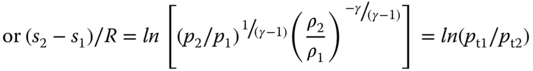
Using perfect gas laws, entropy change process through shock is an adiabatic process, as follows.

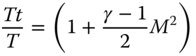
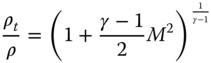
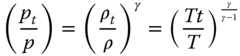
When velocity is stagnated to zero (say in the hole of a pitot tube), then the following equations can be derived for isentropic process. Subscript ‘t’ represents a stagnation property, which is also known as the ‘total’ condition. The equations represent point properties, that is, they are valid at any point of a streamline (γ stands for the ratio of specific heat and M is for Mach number).

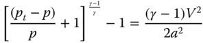
The conservation equations yield many other significant equations. In any streamline of a flow process, the conservation laws exchange pressure energy with kinetic energy. In other words, if the velocity at a point is increased, then the pressure at that point falls and vice versa (i.e. Bernoulli's and Euler's equations). The following are a few more important equations. At stagnation, the total pressure, pt, is given.
or p + ρV2/2 = constant = pt
Clearly, at any point, if the velocity is increased, then the pressure will fall to maintain conservation. This is the crux of lift generation: the upper surface has lower pressure than the lower surface. For compressible isentropic flow, Euler's (Bernoulli's) equation gives the following:
There are other important relations using thermodynamic properties, as follows.
From the gas laws (combining Charles Law and Boyle's Law), the equation for state of gas for unit mass is ![]() where for air
where for air
where Cp = 1004.68 m2 s−2 K−1, Cv = 717.63 m2 s−2 K−1,
Gas constant, R = 287.053 m2 s−2 K−1, Universal Gas constant, R = 8314.32 J (K kmol)−1
Mean molecular mass of air (28.96442 kg kmol−1)

C.3 Supersonic Aerodynamics
Some supersonic 2D relations are given next and Figure C.1 depicts normal and oblique shocks. Upstream flow properties are represented by subscript ‘1’ and downstream by subscript ‘2’. The process across a shock is adiabatic, therefore total energy remains invariant; that is, Tt1 = Tt2.
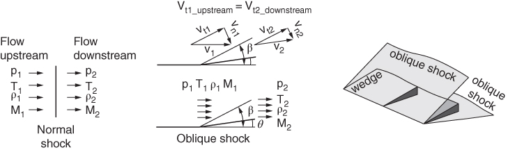
Figure C.1 Shock waves.
C.4 Normal Shock
In this situation, relations between upstream and downstream are unique and do not depend on geometry. If upstream conditions are known, then the downstream properties can be computed from the following relations.

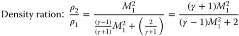
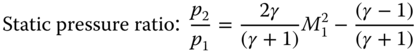
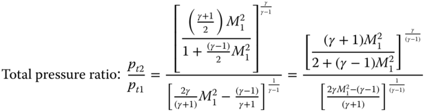
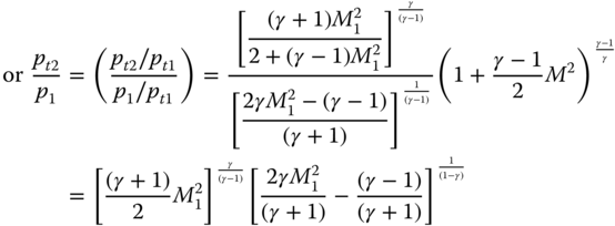
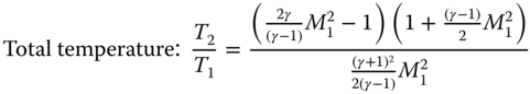
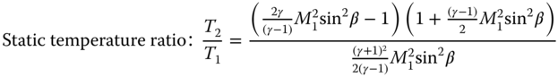
Once the Mach numbers are known, the static temperatures each side of normal shock can be computed from the isentropic relation given in Equation C.2.
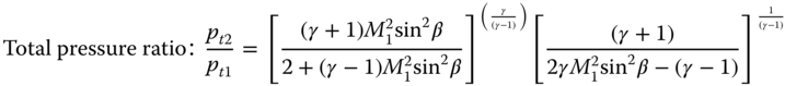
C.5 Oblique Shock
The physics of 2D supersonic flow past a planar surface and 3D flow past body of revolution differs. In the case of 2D wedge, the flow has two degrees of freedom, one along the flow and the other perpendicular to the flow. But in the case of 3D cone, the flow has three degrees of freedom, the third dimension moving laterally. The difference shows in the physics of flow as the shock strength weaker for the cone flow and also have smaller shock angle for the same subtended object angle at the same free‐stream Mach number. This can be checked out in the graphs given next.
A pressure pulse moving through air at speeds higher than the speed of sound will develop as a weak wave pressure cone known as Mach wave. The 2D projection of the Mach wave will have the angle, μ, measured from the centreline. This is a measure of speed and can be computed as follows.
where μ is a characteristic angle associated with the Mach wave in a limiting sense without any discontinuity in the flow field. In practice, all real objects will have some thickness that will deflect airflow as shown in Figure C.1, in which the object in a wedge shape of angle θ creates a shock wave of angle β, which is always higher than μ; that is, β > μ. A shock wave creates a discontinuity across it and is formed by the coalescing of successive Mach waves in the process of flow being deflected. For a given deflection angle, θ, the shock angle, β, can be obtained by the relation given in Equation C.23.
C.6 Supersonic Flow Past a 2D Wedge
Figure C.1, shows the supersonic flow past a wedge shaped object of angle θ creating a shock wave of angle, β. In this situation, relations between upstream and downstream depend on geometry of deflection angle θ and free upstream Mach number M1 develop an oblique shock angle, β. Higher the upstream Mach number M1 lowers the oblique shock angle, β. For the same free upstream Mach number M1, loss through oblique shock is less than normal shock. The relation between free stream Mach number M1, deflection angle θ, and oblique shock angle, β, can be obtained from the following relation.
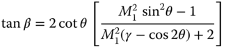
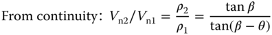
Normal velocities Vn1 and Vn2 on oblique shock can be treated as normal shock. In that case, substitute M1sinβ for M1 in Eqs. C.1 to C.2 obtain relations between properties across oblique shock.


Downstream Mach number: 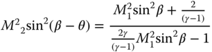
The relation between Mach number M1, deflection angle θ, and oblique shock angle, β are plotted in Figure C.2. It is recommended readers use the graphs in Figure C.2. These graphs will prove easier to get results to the extent they will be used in this book. Section 4.13 indicates that the complexities involved in supersonic aircraft design are beyond the scope of this book. However, some introductory treatment is carried out to make readers aware of the associated considerations required to design supersonic aircraft.

Figure C.2 Shock wave properties.
C.7 Supersonic Flow Past 3D Cone
Supersonic flow physics past 3D bodies differs from 2D planar bodies and therefore Equations (3.23) to (3.28) cannot be used.
Supersonic/hypersonic nose of aircraft and rockets are bodies of revolution resembling an ogive shape. To obtain shock wave properties over an ogive shape is relatively difficult. To simplify, the front portion of an ogive is approximated as a cone and the graphs given in Figure C.3 may be used for initial approximation.

Figure C.3 Properties of shock waves past a 3D cone.
Section 4.12 discusses supersonic wing design.
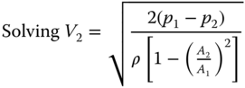
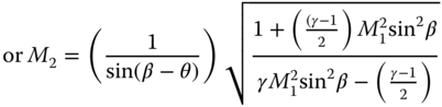
C.8 Incompressible Low Speed Wind Tunnel (Open Circuit)
Refer to the Figure C.4. Let ρ, A and V be the density, cross sectional area and velocity in a settling chamber with subscript 1 and in a test section with subscript 2, respectively. The contraction ratio of the wind tunnel is defined by A1/A2.
Figure C.4 Open circuit low speed wind tunnel.
From conservation of mass flow, m = ρ1A1V1 = ρ2A2V2 (Eq. C.1)
Being incompressible, A1V1 = A2V2
Using Bernoulli's theorem (Eq. C.10) p1 + ρV12/2 = p2 + ρV22/2 (ρ1 = ρ2 = ρ, incompressible)