10
Aircraft Weight and Centre of Gravity Estimation
10.1 Overview
An aircraft must ascend to heights by defying gravity and sustaining the tiring task of cruise – naturally, this is weight‐sensitive. Anyone who has climbed a hill knows about this experience, especially if one has to carry baggage. An inanimate aircraft is no exception; its performance suffers by carrying unnecessary mass (i.e. weight). At the conceptual design stage, aircraft designers have a daunting task of creating a structure not only at a low weight but also at a low cost, without sacrificing safety. Engineers also must be accurate in weight estimation well ahead of manufacture. This chapter presents a formal method to predict an aircraft and its component mass (i.e. weight), which results in locating the centre of gravity (CG) during the conceptual design phase. The aircraft inertia estimation is not within the scope of this book, except finding the area moment of inertia in Chapter 19.
In the past, in the UK and the USA, aircraft mass was expressed in foot pound system (FPS) units in pounds (lbm) and weight in the same pound terminology (lbf), a product of acceleration due to gravity and mass. This may create some confusion to those who are starting to use them for the first time. With the use of kg as mass in the System Internationale (SI), the unit for weight is a newton, which is calculated as the mass multiplied by gravitational acceleration (9.81 m s−2). This book uses both the FPS and SI systems; sometimes interchangeably.
Aircraft weight depends on the materials used for its manufacture. As stated previously, aircraft conceptual designers must have broad‐based knowledge in all aspects of technology; in this case, they must have a sound knowledge of material properties (e.g. strength‐to‐weight and strength‐to‐cost ratios). Higher strength‐to‐weight and strength‐to‐cost ratios are the desired qualities, but they act in opposition. Higher strength‐to‐weight ratio material is more expensive, and designers must stay current in materials technology to choose the best compromises. Chapter 19 is devoted to aircraft materials and structures.
In the early days, designers had no choice but to use the best quality wood for aircraft construction material. Today, it is not a viable option for the type of load encountered. Good quality wood has become expensive and also poses an environmental issue. Fortunately, the advent of duralumin (i.e. an aluminium alloy) in the 1930s resolved the problem, providing a considerably higher strength‐to‐weight ratio than wood. Having a mass‐produced aluminium alloy also offers a lower material cost‐to‐strength ratio. Wood is easier to work with, having a low manufacturing infrastructure suitable for homebuilt aircraft, but other civil and military aircraft use predominantly metal alloys and composites. The last two decades have seen a growing use of composite material and more exotic metal alloys offer still better strength‐to‐weight ratios.
Composites are basically fabric and resin bonded together, generally formed to shape in moulds. The manufacturing process associated with composites is yet to achieve the quality and consistency of metal; hence, at this point, the certifying authorities are compelled to apply reduced values of stress levels to allow for damage tolerance and environmental issues, as well as to keep the factor of safety at 1.5. The manufacturing process also plays a role in deciding the allowable stress level. These considerations can erode the benefits of weight savings. Research on new material, whether metal alloys (e.g. lithium‐aluminium and beryllium alloy) or composites (e.g. fabric and resin) or their hybrids, is an area where there is potential to reduce aircraft weight and cost. New materials are still relatively expensive, and they are steadily improving in both strength and lower costs.
This chapter covers the following topics:
- Section 10.2: Aircraft Mass, Component Mass and CG Position
- Section 10.3: Parameters that Act as Drivers for Aircraft Mass
- Section 10.4: Aircraft Mass Breakdown Sequence
- Section 10.5: Desirable CG Location Relative to Aircraft
- Section 10.6: Aircraft Mass Decomposed into Component Groups
- Section 10.7: Aircraft Component Mass Estimation Methods
- Section 10.8: Civil Aircraft Rapid Mass Estimation Method
- Section 10.9: Civil Aircraft Graphical Mass Estimation Method
- Section 10.10: Civil Aircraft Semi‐Empirical Mass Estimation Method
- Section 10.11: Bizjet Example
- Section 10.12: Methodology to Establish Aircraft CG with a Bizjet Example
- Section 10.13: Military Aircraft Rapid Mass Estimation Method
- Section 10.14: Military Aircraft Graphical Method for Mass Estimation
- Section 10.15: Military Aircraft Semi‐Empirical Mass Estimation Method
- Section 10.16: AJT and CAS Examples (Military Aircraft)
- Section 10.17: Methodology to Locate Aircraft CG with AJT and CAS Examples
- Section 10.18: TPT and COIN Examples
10.1.1 Coursework Content
The coursework task continues linearly with the examples worked out thus far. Readers must estimate aircraft component mass, which gives the aircraft mass and its CG location. This is an important aspect of aircraft design because it determines aircraft performance, stability and control behaviour.
Experience in the industry has shown that weight can only grow. Aircraft performance is extremely sensitive to weight because it must defy gravity. Aerodynamicists want the least weight, whereas stress engineers want the component to be strong so that it will not fail and have the tendency to beef‐up a structure. The structure must go through ground tests when revisions may be required. It is easy to omit an item (there are thousands) in weights estimation. Most aeronautical companies have a special division to manage weights by weights‐control engineers – a difficult task to perform. The aircraft operators also have loadmasters to ensure loading of aircraft for safe operation for the full operational envelope, on ground and in flight.
10.2 Introduction
Because aircraft performance and stability depends on aircraft weight and the CG location, the aircraft weight and its CG position are paramount in configuring an aircraft. The success of a new aircraft design depends considerably on how accurately its weight (mass) is estimated. A pessimistic prediction masks product superiority and an optimistic estimation compromises structural integrity. A pessimistic prediction ends up as a lighter aircraft showing better performance in prototype flight tests and is easy to correct, but an optimistic prediction may come out with a heavier aircraft and may fail to meet the performance requirements when it may prove expensive to lighten the weight by compromising structural integrity.
Once an aircraft is manufactured, the component weights can be easily determined by actual weighing. The aircraft CG then can be accurately determined. However, the problem is in predicting weight and the CG is at the conceptual design stage, before the aircraft is built. When the first prototype is built, the weights engineers have the opportunity to verify the predictions – typically, a four‐year wait! Many of the discrepancies result from design changes; therefore, weights engineers must be kept informed in order to revise their estimations. It is a continuous process as long as the product is well supported after the design is completed.
Mass is the product of the solid volume and average density. For an aircraft component (e.g. wing assembled from a multitude of parts and fasteners), it is a laborious process to compute volumes of all those odd‐shaped parts. In fact, the difficulty is that the mass prediction of complex components is not easily amenable to theoretical derivations. The typical approach to estimate weights at the conceptual design stage is to use semi‐empirical relationships based on theory and statistical data of previously manufactured component masses (a 3D computer aided drawing (CAD) model of parts provides the volume but may not be available in the conceptual design stage).
The mass of each component depends on its load‐bearing characteristics, which in turn depend on the operational envelope (i.e. the V‐n diagram). Each manufacturer has a methodology developed over time from the statistics of their past products combined with the physical laws regarding mass required for the geometry to sustain the load in question. These semi‐empirical relations are proprietary information and are not available in the public domain. All manufacturers have developed mass‐prediction relationships yielding satisfactory results (e.g. an accuracy of less than ±3% for the type of technology used). The semi‐empirical relations of various origins indicate similarity in the physical laws but differ in associated coefficients and indices to suit their application domain (e.g. military or civil, metal, structural and manufacturing philosophy and/or level of desired accuracy). Nowadays, computers are used to predict weight through solid modelling – this is in conjunction with semi‐empirical relations. The industry uses more complex forms with involved and intricate manipulations that are not easy to work within a classroom.
The fact is that, no matter how complex academia may propose semi‐empirical relations to be to improve accuracy in predicting component mass, it may fall short in supplanting the relationship available in industry based on actual data. Out of necessity, the industry must keep its findings ‘commercial in confidence’. At best, industry may interact with academia for mutual benefit. An early publication by Torenbeek [1] with his semi‐empirical relations is still widely used in academic circles. Roskam [2] presented three methods (i.e. Torenbeek, Cessna and US DATCOM) that clearly demonstrate the difficulty in predicting mass. Roskam's book presents updated semi‐empirical relations corroborated with civil aircraft data showing satisfactory agreement. The equations are not complex – complexity does not serve the purpose of coursework. Readers will have to use industrial formulae when they join a company. This chapter explains the reasons associated with formulating the relationships to ensure that readers understand the semi‐empirical relations used in the industry.
The authors recommend the publications by the Society of Allied Weights Engineers (SAWE) (US) as a good source for obtaining semi‐empirical relations in the public domain. Some of the relations presented herein are taken from SAWE, Torenbeek, Sechler, Roskam, Niu and Jenkinson ([1–6]). Some of the equations are modified by the authors. It is recommended that readers collect as much component weight data as possible from various manufacturers (both civil and military) to check and modify the correlations and to improvise if necessary. Revision of mass (i.e. weight) data is a continuous process. In each project phase, the weight estimation method is refined to better accuracy. Actual mass is known when components are manufactured, providing an opportunity to assess the mass‐prediction methodology. Although strength testing of major aircraft components is a mandatory regulatory requirement before the first flight, structural‐fatigue testing continues after many aircraft are already in operation. By the time results are known, it may not prove cost‐effective to extensively modify an overdesigned structural member until a major retrofit upgrading is implemented at a later date.
The unavoidable tendency is that aircraft weight grows over time primarily due to modifications (e.g. reinforcements and additions of new components per user requirements). Provision needs to be made at the conceptual stage to manage the weight growth. There are several ways to achieve this, the simplest way is to tweak the engine to produce slightly increased thrust (typically a 1% thrust increase for 4% weight growth – this should prove sufficient in the majority of cases).
The importance of the Six‐Sigma approach to make a design right the first time is significant to weights engineers. Many projects have suffered because of prototypes that were heavier than prediction or even experienced component failure in operation resulting in weight growth. The importance of weight prediction should not be underestimated due to not having an analytical approach involving high‐level mathematical complexity, as in the case of aerodynamics. Correct weight estimation and its control are vital to aircraft design. One cannot fault stress engineers for their conservatism in ensuring structural integrity – lives depend on it. Weight‐control engineers check for discrepancies throughout project development.
Mass‐prediction methodology starts with component weight estimation categorised into established groups, as described in Section 10.6. The methodology culminates in overall aircraft weight and locating the CG and its range of variation that can occur in operation. Aircraft inertias are required to assess dynamic behaviour in response to control input but then they are not needed until completion of the conceptual design study – hence, inertia is not addressed in this book. Iteration of the aircraft configuration is required after the CG is located because it is unlikely to coincide with the position guesstimated from statistics.
10.2.1 From ‘Concept Definition’ to ‘Concept Finalisation’
Progress of aircraft conceptual design study up to Chapter 9 led to presenting a preliminary configuration based on confident ‘guesstimates’ of maximum takeoff mass (MTOM), wing and other geometric parameters, and engine size from the statistics of past designs. From this chapter and onwards, work progresses towards refinement to accurate values as much as is possible, through iterations to update design to a better definition to arrive at the end to concept definition, in order to freeze aircraft to, that is, concept finalisation in Chapter 14. This completes Phase I of the project and enters into Phase II, the ‘Detailed Design Phase’; beyond the scope of this book.
In this chapter, aircraft and component weight estimation are carried out using reliable and well‐established semi‐empirical formulae, followed by establishing the aircraft CG position. It is expected that the estimated MTOM and CG position will be different from the guessed values. This will necessitate returning to a point to iterate through the subsequent stages to arrive at an improved concept definition. The iterative process may require repositioning of wing and undercarriage with respect to the fuselage. The last iteration will be after the aircraft is sized (Chapter 14) with a matched engine that could necessitate altering of wing reference area (like zooming in/out) yet maintain geometric parameters of sweep, taper ratio, dihedral and twist unaffected. Change of wing reference area will also affect empennage reference areas. Geometric changes will also change aircraft drag affecting engine size. All these changes will also change aircraft component weights. Therefore, at least, another iteration is required to fine‐tune aircraft configuration to, that is, concept finalisation, to freeze the design. Experience designers can minimise iterative process. This book avoids iterations to save from repetitive work.
Once again, the authors recommend that the readers prepare spreadsheets for repeated calculations because iterations will ensue after the CG is established and the aircraft is sized.
10.3 The Weight Drivers
The factors that drive aircraft weight are listed herein. Aircraft material properties given are typical for comparing relative merits. Material elasticity, E, and density, ρ, provide the strength‐to‐weight ratio. In the alloys and material categories, there is variation. Chapter 19 deals with aircraft materials and structures.
- Weight is proportionate to size, indicated by geometry (i.e. length, area and volume).
- Weight depends on internal structural‐member density – that is, the denser, the heavier.
- Weight depends on a specified limit‐load factor n (see Chapter 17) for structural integrity.
- Fuselage weight depends on pressurisation, engine and undercarriage mounts, doors and so forth.
- Lifting surface weight depends on the loading, fuel carried, engine and undercarriage mounts and so forth.
- Weight depends on the choice of material. There are seven primary types used in aircraft, as follows:
- (a) Aluminium alloy (a wide variety is available – in general, the least expensive) typical E = 11 × 106 lb in.−2; typical density = 0.1 lb in.−3
- (b) Aluminium–lithium alloy (fewer types available – relatively more expensive)
typical E = 12 × 106 lb in.−2; typical density = 0.09 lb in.−3
- (c) Stainless‐steel alloy (hot components around engine – relatively inexpensive)
typical E = 30 × 106 lb in.−2; typical density = 0.29 lb in.−3
- (d) Titanium alloy (hot components around engine – medium‐priced but lighter)
typical E = 16 × 106 lb in.−2; typical density = 0.16 lb in.−3
- (e) Composite type varies (e.g. fibreglass, carbon fibre and Kevlar); therefore, there is a wide variety in elasticity and density (price varies from inexpensive to expensive).
- (f) Hybrid (metal and composite ‘sandwich’ – very expensive, e.g. Glare).
- (g) Wood (rarely used except for homebuilt aircraft; is not discussed in this book).
Figure 10.1 Aircraft weights breakdown.
The use of composites is increasing, as evidenced in current designs. In this book, the primary load‐bearing structures are constructed of metal; secondary structures (e.g. floorboard and flaps) could be made from composites. On the conservative side, it generally is assumed that composites and/or new alloys allow about 10–15% weight saving of the manufacturer's empty mass (MEM) for civil aircraft and about 15–25% of the MEM for military aircraft. Although composites are used in higher percentages, this book remains conservative in approach. All‐composite aircraft have been manufactured (mostly small aircraft), although only few in number (except small aircraft). The metal‐composite sandwich is used in the Airbus380 and Russia has used aluminium–lithium alloys. In this book, weight change as the consequences of using newer material is addressed by applying factors.
The design drivers for civil aircraft have always been safety and economy. Competition within these constraints kept civil aircraft designs similar to one another.
10.4 Aircraft Mass (Weight) Breakdown
Given next and in Figure 10.1 are definitions of various groups of aircraft mass (weight).
MEM (manufacturer's empty mass)
This is the mass of a finished aircraft as it rolls out of the factory before it is taken to a flight hangar for the first flight.
The aircraft is now ready for operation (residual fuel from the previous flight remains).
The MTOM is the reference mass loaded to the rated maximum design limit. This is also known as the brake release mass (BRM) ready to takeoff. (Not all takeoffs are at MTOM.)
Aircraft are allowed to carry a measured amount of additional fuel for taxiing to the end of the runway, ready for takeoff at the BRM (MTOM). This additional fuel mass would result in the aircraft exceeding the MTOM to the maximum ramp mass (MRM). Taxiing fuel for midsized aircraft would be approximately 100 kg and it must be consumed before the takeoff roll is initiated – the extra fuel for taxiing is not available for the range calculation. On busy airfields, the waiting period in line for takeoff could extend to more than an hour in extreme situations. MRM is also known as the maximum taxi mass (MTM) and is heavier than the MTOM.
The maximum permissible landing mass is 0.95 MTOM. Fuel dumping is not allowed around built‐up areas. Aircraft can land at any mass heavier than design landing mass (DLM), when short hop consecutive sorties are carried out without refuelling.
10.5 Aircraft CG and Neutral Point Positions
Proper distribution of mass (i.e. weight) over the aircraft geometry is key to establishing the CG. It is important for locating the wing, undercarriage, engine and empennage for aircraft stability and control. The convenient method is to first estimate each component weight separately and then position them to satisfy the CG for the maximum takeoff weight (MTOW).
Fuel loads and payloads are variable quantities; hence, the CG position varies relative to overall geometry. Each combination of fuel and payload results in a CG position. The position of CG with respect to aircraft is an important consideration for operations on ground and in flight. There are two extreme CG positions to travel for safe operation. A typical aircraft CG margin that affects aircraft operation is shown in Figure 10.2. On ground, the aircraft should not trip over longitudinally and laterally (see Chapter 9). In flight, the aircraft must remain stable for the full flight envelope. A similar plot can be made for lateral CG movement for the consideration of turn‐over issues (not shown here).

Figure 10.2 Aircraft CG limits.
Figure 10.3 Aircraft CG limits travel – range of CG variations. (a) ‘Potato’ curve showing the horizontal limits (shaded area) and (b) vertical limits.
Aircraft operators, civil or military, have a team of ground crew who plans and computes the permissible load for the mission sortie. For civil operations, the appropriate containers and packaging are used. For military aircraft, it is the armaments and various types of pods and so on. The team is headed by the ‘Loadmaster’ who is responsible fuel and cargo/payload loading sequence to ensure safe operation on ground and in flight.
Figure 10.3 shows variations in CG positions for the full range of combinations. Because it resembles the shape of a potato, the CG variation for all loading conditions is sometimes called the ‘potato curve’; also embedded in Figure 10.2. Designers must ensure that at no time during loading up to the MTOM does the CG position exceed the loading limits endangering the aircraft to tip over on any side. Loading must be accomplished under supervision. Whereas passengers have free choice in seating, cargo and fuel loading are done in prescribed sequences, with options.
It has been observed that passengers first choose window seats and then, depending on the number of abreast seating, the second choice is made. Figure 10.3a shows the window seating first and the aisle seating last; note the boundaries of front and aft limits. Cargo and fuel loading is accomplished on a schedule with the locus of CG travel in lines. In the figure, the CG of the operator's empty mass (OEM) is at the rear, indicating that the aircraft has aft‐mounted engines. For wing‐mounted engines, the CG at the OEM moves forward, making the potato curve more erect.
Figure 10.3b represents a typical civil aircraft loading map, which indicates the CG travel to ensure that the aircraft remains in balance within horizontal and vertical limits. Loading starts at the OEM point; if the passengers boarding first opt to sit in the aft end, then the CG can move beyond the airborne aft limit, but it must remain within the ground limit. Therefore, initial forward cargo loading should precede passenger boarding; an early filling of the forward tank fuel is also desirable.
10.5.1 Neutral Point, NP
Aircraft NP is the aerodynamic centre of a weightless aircraft (see Section 3.7). NP is the point where dM/dα is constant, that is, aircraft pitching moment is invariant to attitude changes. In‐flight CG has to take into account of the influence wing position relative to fuselage and H‐tail size that determine the aircraft aerodynamic centre, a shape dependent aerodynamic parameter. Therefore, the position of NP shifts if external geometric shape changes, for example, between clean and dirty (hi‐lift devices and/or undercarriage are in extended position) conditions. Also, the position of CG changes depending on the fuel and payload/cargo loading status; seen as CG travel. The CG position with respect to the aircraft neutral is an important consideration to maintain aircraft stability.
Figure 10.4 shows that the aircraft NP moves backward near ground during field performance (takeoff and landing at dirty configuration) due to the flow field being affected by ground constraints. There is also movement of the CG location depending on the loading (i.e. fuel and/or passengers). It must be ensured that the pre‐flight aft‐most CG location is forward of the in‐flight NP centre by a convenient margin, which should be as low as possible to minimise trim. The distance between aircraft CG and the aircraft NP is known as the stability margin of the aircraft. (To repeat that the main‐wheel contact point (and strut line) is aft of the aft‐most CG, the subtending angle, β, should be greater than the fuselage‐rotation angle, γ, as described in Section 9.6.)
Figure 10.4 Aircraft CG position showing the stability margin.
10.5.2 Aircraft CG Travel
Aircraft approaches to unstable flight as CG moves close to the NP. CG behind NP makes an aircraft unstable (see Chapter 18). The designers must ensure safe operation for the full operating envelope. (Note that an aircraft can be flown at neutral stability. This requires the pilot to struggle all the time to maintain steady attitude that will tire them out, which is not a safe way to fly. A bicycle ride is a good example where one has to learn to stay in balance.) Advanced military combat aircraft with Fly‐by‐Wire (FBW) technology can have relaxed static stability to provide quicker responses. That is, the margin between the aft‐most CG and the in‐flight NP is reduced (it may be even slightly negative), but design considerations relative to the undercarriage position remain unaffected. The following are some points for consideration that determine the extremities of CG travel.
Forward‐Most CG Position
- If the aircraft is loaded to MTOW or close to it in a manner that makes CG stay forward then load on the nose becomes high and steering problems could show up. The nose gear limit line for high aircraft is shown in Figure 10.2.
- Aircraft in a dirty configuration with a forward CG position have a high nose down moment requiring adequate elevator power with downward force to keep the aircraft in balance to maintain the desirable attitude. In the case of bad design, trim may run out at the landing configuration with a forward CG when the pilot may not be able to raise the nose up sufficiently to the landing attitude.
- A larger sized H‐tail may overcome this problem at the expense of high stick force. It can now be realised that a compromise is required to size the H‐tail.
Aft‐Most CG Position
- The aft‐most CG limit is concerned with aircraft safety. As the aircraft CG moves closer to the NP, which must be always behind, the pitch actuation force becomes lighter and the aircraft becomes more responsive with the pilot requiring little force to change pitch attitude. In loose terms, the control stick feels lighter. It suites military pilots, but there is a limit beyond which the pilot will have to struggle with constant attention. A limit has to be given for safe operation, which is the aft limit of the CG.
- During field performance, aft‐most CG at a high load will have a high main gear load (Section 9.7). The main gear limit line for a highly loaded aircraft is shown in Figure 10.2.
- For pitch stability consideration, a minimum stability margin has to be given suited to the H‐tail size. Trim drag is minimum at the aft‐most CG position.
CG at MTOM is not necessarily at the forward‐most limit. Similarly, the CG of an empty aircraft at OEW (Operator's Empty Weight) is not necessarily at the aft‐most position. The CG is always forward of the NP point. The loadmaster's responsibility is to make sure the aircraft CG travel stays within the specified limits for the full operational envelope.
Initially, locations of some of the components (e.g. the wing) were arbitrarily chosen based on designers' past experience, which works well (see Chapter 8). Iterations are required that, in turn, may force any or all of the components to be repositioned. There is flexibility to fine‐tune the CG position by moving heavy units (e.g. batteries and fuel storage positions). It is desirable to position the payload around the CG so that any variation will have the least effect on CG movement. Fuel storage should be distributed to ensure the least CG movement; if this is not possible, then an in‐flight fuel transfer is necessary to shift weight to maintain the desired CG position (as in the case of supersonic Concorde).
10.6 Aircraft Component Groups
The recognised groups of aircraft components are listed in exhaustive detail in the Aircraft Transport Associations (ATAs) publication. This section presents consolidated, generalised groups (for both civil and military aircraft) suitable for studies in the conceptual design phase. Both aircraft classes have similar nomenclature; the differences in military aircraft follow the common listings. Each group includes subgroups of the system at the next level. Care must be taken that items are not duplicated – accurate book‐keeping is essential. For example, although the passenger seats are installed in the fuselage, for book‐keeping purposes, the fuselage shell and seats are counted separately.
10.6.1 Aircraft Components
- Fuselage group (MFU)
- Wing group (MW) – includes all structural items, for example, flaps, winglets and so on
- Horizontal tail group (MHT)
- Vertical tail group (MVT)
- Nacelle group (MN and MPY – nacelle and pylon)
- Undercarriage group (MUC)
- Miscellaneous (MMISC) – dorsal, ventral fins and so on
Military aircraft have the following to be accounted for:
- Fixed armament (MFARM), for example, internal guns and so on
- Pylon (MPYL) – to carry armament load/drop tank.
This is the basic structure of the aircraft, for example, the fuselage shell (seats are separated under furnishing group) and so on.
- Dry equipped engine (ME)
- Thrust reverser (MTR)
- Engine control system (MEC)
- Fuel system (MFS)
- Engine oil system (MOI)
Military aircraft have the following to be accounted for:
- Retarding devise (MRD), for example, brake parachute (MRD).
These come as a package and are items dedicated to power plant installation. They are mostly bought‐out items supplied by specialists.
- Environmental control system (MECS)
- Flight control system (MFC)
- Hydraulic/pneumatic system (MHP) – sometimes lumped in with other systems
- Electric system (MELEC)
- Instrument system (MINS)
- Avionics system (MAV)
- Oxygen system (MOX).
Military aircraft have the following to be accounted for:
- Ejection seat system – this is no more treated as furnishing (MEJ).
A wide variety of equipment, these are all vendor‐supplied bought‐out items.
- Seat, galleys and other furnishing (MSEAT)
- Paints (MPN).
Note that most of the weight goes to the fuselage, yet this is itemised under a different heading. Paints can be quite heavy. A well‐covered B737 with airline livery can use up 75 kg of paint.
Contingencies (MCONT)
- Contingencies (MCONT) – a margin to allow unspecific weight growth
MEM – the total of these items.
This is the weight of the complete aircraft coming out from the production line for the first time to be airborne. The following items are added to MEM to obtain OEM.
- Crew – Flight and cabin crews (MCREW)
- Consumables – Food, water and so on. (MCON)
(long duration military sortie have consumables for the crew)
OEM – aircraft is now ready for operation.
To make it sortie ready, add the payload and requisite fuel to obtain MRM.
- Fuel (MFUEL) – for the design range, which may not fill all tanks
Civil aircraft specific payload is the passengers and/or cargo is the following:
- Payload (MPL passengers @ 90 kg per passenger – includes baggage)
Military aircraft specific payload is the armament/electronic devices as the following:
- Armaments (MARM) – missiles, bombs, firing rounds, drop tanks, electronic pods and so on.
MTOM (Maximum Takeoff Mass) = (MRM – taxi fuel)
That is the aircraft at the edge of runway ready to takeoff.
Civil Aircraft MTOM weight is the sum of weights of all component groups as totalled next.

where subscript ‘i’ stands for each component group listed here.
For civil aircraft:
For military aircraft:
10.7 Aircraft Component Mass Estimation
Mass estimation at the conceptual design stage must be predicted well in advance of detailed drawings of the parts being prepared. Statistical fitment of data from the past designs is the means to predict component mass at the conceptual design phase. The new designs strive for improvement; therefore, statistical estimation is the starting point. During the conceptual design stage, iterations are necessary when the configuration changes. Typically, there are three ways to make mass (i.e. weight) estimations at the conceptual design stage:
- Mass fraction method. This method relies on the statistical average of mass (Section 10.8). The mass is expressed in terms of percentage (alternatively, as a fraction) of the MTOM. All items should total 100% of the MTOM; this also can be expressed in terms of mass per wing area (i.e. component wing loading). This mass fraction method is accomplished at the cost of considerable approximation. This method is useful in setting up an equation by taking mass fractions as parameters to make analytical studies. This book bypasses the mass fraction method except to tabulate the range of mass fractions in Section 10.8.
- Graphical method. This method consists of plotting component weights of various aircraft already manufactured to fit into a regression curve. The graphical method does not provide fine resolution but it is the fastest. It is difficult to capture the technology level (and types of material) used because there is considerable dispersion. Obtaining details of component mass for statistical analysis from various industries is difficult.
- Semi‐empirical method. This method is a considerable improvement in that it uses semi‐empirical relations derived from a theoretical foundation and is backed by actual data that have been correlated statistically. The indices and factors in the semi‐empirical method can be refined to incorporate the technology level and types of material used. The expressions can be represented graphically, with separate graphs for each class. When grouped together in a generalised manner, they are the graphs in the graphical method described previously.
The three methods are addressed in more detail in the Sections 10.8–10.10. While the first two methods of component mass estimation provide a starting point for Phase I, it will be necessary to refine the estimation of semi‐empirical weight estimation equations.
10.7.1 Use of Semi‐Empirical Weight Relations versus Use of Weight Fractions
Section 1.11.2 discusses the merit of using the semi‐empirical weights formulae. The weight fraction data and related graphs are generated from the statistics of the latest aircraft in operation may not be close enough. Statistical based weight fractions data offer a good check to examine if the results obtained using the semi‐empirical weights formulae are in agreement or not. Industries maintain databases of existing aircraft and possible competition aircraft to give some idea of what is expected and serve to initiate the conceptual design study and make comparisons. After that, the typical trend in industry is to use their in‐house semi‐empirical weights formulae for aircraft components weight estimation with substantiated accuracy within 5% to begin with and gets refined to less than to 2% before the final assembly of the first aircraft is completed. Once manufactured, accurate weights data for components and the whole aircraft can be quickly weighed to obtain the exact value.
10.7.1.1 Weight Fraction Method
Initial weight estimates using weights will, however, offer rather crude values as modern aircraft are increasingly incorporating newer materials for which there may not sufficient data available. Tables 10.1–10.3 give the component weight/mass fractions with respect to MTOM. While the use of weight fractions is reasonable to consider, it will be more convenient to prepare graphs as given in Figure 10.5 for rapid estimation with an error band no less than using the mass fractions. Visual inspection of the graphs allows intelligently deselecting extreme points to narrow the error band to improve results within the class of aircraft. The authors think that the classroom exercises should generate their own data within the category of aircraft closest to their project and plot graphs that will offer the tighter error band with the latest data. Once the preliminary aircraft configuration is established using statistics, it is recommended to use the semi‐empirical formulae in the next iteration instead of weight fractions to obtain better accuracy. For this reason, although the weight fraction data are given in Tables 10.1--10.3, these are not used in the worked‐out examples.
Table 10.1 Smaller aircraft mass fraction (typically less than around 19 passengers – two‐abreast seating).
| Group | Small piston aircraft (one piston) | Agricultural aircraft | Small aircraft: two engine (Bizjet utility) | |||
| One engine | Two engine | One piston | Turboprop | Turbofan | ||
| Fuselage | Ffu = MF/MTOM | 12–15 | 6–10 | 6–8 | 10–11 | 9–11 |
| Wing | Fw = Mw/MTOM | 10–14 | 9–11 | 14–16 | 10–12 | 9–12 |
| H‐tail | Fht = Mht/MTOM | 1.5–2.5 | 1.8–2.2 | 1.5–2 | 1.5–2 | 1.4–1.8 |
| V‐tail | Fvt = Mvt/MTOM | 1–1.5 | 1.4–1.6 | 1–1.4 | 1–1.5 | 0.8–1 |
| Nacelle | Fn = Mn/MTOM | 1–1.5 | 1.5–2 | 1.2–1.5 | 1.5–1.8 | 1.4–1.8 |
| Pylon | Fpy = Mpy/MTOM | 0 | 0 | 0 | 0.4–0.5 | 0.5–0.8 |
| Undercarriage | Fuc = Muc/MTOM | 4–6 | 4–6 | 4–5 | 4–6 | 3–5 |
| Engine | FE = ME/MTOM | 11–16 | 18–20 | 12–15 | 7–10 | 7–9 |
| Thrust rev. | Ftr = Mtr/MTOM | 0 | 0 | 0 | 0 | 0 |
| Engine con. | Fec = Mec/MTOM | 1.5–2.5 | 2–3 | 1–2 | 1.5–2 | 1.7–2 |
| Fuel sys. | Ffs = Mfs/MTOM | 0.7–1.2 | 1.4–1.8 | 1–1.4 | 1–1.2 | 1.2–1.5 |
| Oil sys. | Fos = Mos/MTOM | 0.1–0.3 | 0.25–0.4 | 0.1–0.3 | 0.3–0.5 | 0.3–0.5 |
| APU | 0 | 0 | 0 | 0 | 0 | |
| Flight con. sys | Ffc = Mfc/MTOM | 1.5–2 | 1.4–1.6 | 1–1.5 | 1.5–2 | 1.5–2 |
| Hydr/pneumatic sys | Fhp = Mhp/MTOM | 0–0.3 | 0.3–0.6 | 0–0.3 | 0.5–1.5 | 0.7–1 |
| Electrical | Felc = Melc/MTOM | 1.5–2.5 | 2–3 | 1.5–2 | 2–4 | 2–4 |
| Instrument | Fins = Mins/MTOM | 0.5–1 | 0.5–1 | 0.5–1 | 0.5–1 | 0.8–1.5 |
| Avionics | Fav = Mav/MTOM | 0.2–0.5 | 0.4–0.6 | 0.2–0.4 | 0.3–0.5 | 0.4–0.6 |
| ECS | Fecs = Mecs/MTOM | 0–0.3 | 0.4–0.8 | 0–0.2 | 2–3 | 2–3 |
| Oxygen | Fox = Mox/MTOM | 0–0.2 | 0–0.4 | 0 | 0.3–0.5 | 0.3–0.5 |
| Furnishing | Ffur = Mfur/MTOM | 2–6 | 4–6 | 1–2 | 6–8 | 5–8 |
| Misc. | Fmsc = Mmsc/MTOM | 0–0.5 | 0–0.5 | 0–0.5 | 0–0.5 | 0–0.5 |
| Paint | Fpn = Mpn/MTOM | 0.01 | 0.01 | 0–0.01 | 0.01 | 0.01 |
| Contingency | Fcon = Mcon/MTOM | 1–2 | 1–2 | 0–1 | 1–2 | 1–2 |
| Manufacturer's Empty Weight (MEW) – % | 57–67 | 60–65 | 58–62 | 58–63 | 55–60 | |
| Crew | 6–12 | 6–8 | 4–6 | 1–3 | 1–3 | |
| Consumable | 0–1 | 0–1 | 0 | 1–2 | 1–2 | |
| OEM – % | 65–75 | 65–70 | 62–66 | 60–66 | 58–64 | |
| Payload and fuel are traded | ||||||
| Payload | 12–25 | 12–20 | 20–30 | 15–25 | 15–20 | |
| Fuel | 8–14 | 10–15 | 8–10 | 10–20 | 15–25 | |
| MTOM – % | 100 | 100 | 100 | 100 | 100 | |
| Lighter/smaller aircraft would show the higher side of the mass fraction. | ||||||
Table 10.2 Larger aircraft mass fraction (more than 19 passengers – three‐abreast and above seating).
| Group | RJ/Mid‐size aircraft | Large aircraft | |||
| Two engines | Turbofan | ||||
| Turboprop | Turbofan | Two engine | Four engine | ||
| Fuselage | Ffu = MF/MTOM | 9–11 | 10–12 | 10–12 | 9–11 |
| Wing | Fw = Mw/MTOM | 7–9 | 9–11 | 12–14 | 11–12 |
| H‐tail | Fht = Mht/MTOM | 1.2–1.5 | 1.8–2.2 | 1–1.2 | 1–1.2 |
| V‐tail | Fvt = Mvt/MTOM | 0.6–0.8 | 0.8–1.2 | 0.6–0.8 | 0.7–0.9 |
| Nacelle | Fn = Mn/MTOM | 2.5–3.5 | 1.5–2 | 0.7–0.9 | 0.8–0.9 |
| Pylon | Fpy = Mpy/MTOM | 0–0.5 | 0.5–0.7 | 0.3–0.4 | 0.4–0.5 |
| Undercarriage | Fuc = Muc/MTOM | 4–5 | 3.4–4.5 | 4–6 | 4–5 |
| Engine | FE = ME/MTOM | 8–10 | 6–8 | 5.5–6 | 5.6–6 |
| Thrust rev. | Ftr = Mtr/MTOM | 0 | 0.4–0.6 | 0.7–0.9 | 0.8–1 |
| Engine con. | Fec = Mec/MTOM | 1.5–2 | 0.8–1 | 0.2–0.3 | 0.2–0.3 |
| Fuel sys. | Ffs = Mfs/MTOM | 0.8–1 | 0.7–0.9 | 0.5–0.8 | 0.6–0.8 |
| Oil sys. | Fos = Mos/MTOM | 0.2–0.3 | 0.2–0.3 | 0.3–0.4 | 0.3–0.4 |
| APU | 0–0.1 | 0–0.1 | 0.1 | 0.1 | |
| Flight con. sys | Ffc = Mfc/MTOM | 1–1.2 | 1.4–2 | 1–2 | 1–2 |
| Hydr/pneumatic sys | Fhp = Mhp/MTOM | 0.4–0.6 | 0.6–0.8 | 0.6–1 | 0.5–1 |
| Electrical | Felc = Melc/MTOM | 2–4 | 2–3 | 0.8–1.2 | 0.7–1 |
| Instrument | Fins = Mins/MTOM | 1.5–2 | 1.4–1.8 | 0.3–0.4 | 0.3–0.4 |
| Avionics | Fav = Mav/MTOM | 0.8–1 | 0.9–1.1 | 0.2–0.3 | 0.2–0.3 |
| ECS | Fecs = Mecs/MTOM | 1.2–2.4 | 1–2 | 0.6–0.8 | 0.5–0.8 |
| Oxygen | Fox = Mox/MTOM | 0.3–0.5 | 0.3–0.5 | 0.2–0.3 | 0.2–0.3 |
| Furnishing | Ffur = Mfur/MTOM | 4–6 | 6–8 | 4.5–5.5 | 4.5–5.5 |
| Misc. | Fmsc = Mmsc/MTOM | 0–0.1 | 0–0.1 | 0–0.5 | 0–0.5 |
| Paint | Fpn = Mpn/MTOM | 0.01 | 0.01 | 0.01 | 0.01 |
| Contingency | Fcon = Mcon/MTOM | 0.5–1 | 0.5–1 | 0.5–1 | 0.5–1 |
| MEW – % | 53–55 | 52–55 | 50–54 | 48–50 | |
| Crew | 0.3–0.5 | 0.3–0.5 | 0.4–0.6 | 0.4–0.6 | |
| Consumable | 1.5–2 | 1.5–2 | 1–1.5 | 1–1.5 | |
| OEW – % | 54–56 | 53–56 | 52–55 | 50–52 | |
| Payload and fuel are traded | |||||
| Payload | 15–18 | 12–20 | 18–22 | 18–20 | |
| Fuel | 20–28 | 22–30 | 20–25 | 25–32 | |
| MTOM – % | 100 | 100 | 100 | 100 | |
| Lighter aircraft would show the higher side of the mass fraction. Large turbofan aircraft have wing‐mounted engines. | |||||
Table 10.3 Aircraft component weights data.
| Aircraft | Weight – lb | ||||||||
| MTOW | Fuse | Wing | Emp | Nacelle | Eng. | U/C | n | ||
| Piston‐engined aircraft | |||||||||
| 1. | Cessna 182 | 2 650 | 400 | 238 | 62 | 34 | 417 | 132 | 5.7 |
| 2. | Cessna310A | 4 830 | 319 | 453 | 118 | 129 | 852 | 263 | 5.7 |
| 3. | Beech65 | 7 368 | 601 | 570 | 153 | 285 | 1 008 | 444 | 6.6 |
| 4. | Cessna404 | 8 400 | 610 | 860 | 181 | 284 | 1 000 | 316 | 3.75 |
| 5. | Herald | 37 500 | 2986 | 4365 | 987 | 830 | 1625 | 3.75 | |
| 6. | Convair240 | 43 500 | 4227 | 3943 | 922 | 1213 | 1530 | 3.75 | |
| Gas‐turbine powered aircraft | |||||||||
| 7. | Lear25 | 15 000 | 1575 | 1467 | 361 | 241 | 792 | 584 | 3.75 |
| 8. | Lear45 classa | 20 000 | 2300 | 2056 | 385 | 459 | 1672 | 779 | 3.75 |
| 9. | Jet star | 30 680 | 3491 | 2827 | 879 | 792 | 1750 | 1061 | 3.75 |
| 10. | Fokker27‐100 | 37 500 | 4122 | 4408 | 977 | 628 | 2427 | 1840 | 3.75 |
| 11. | CRJ200 class a | 51 000 | 6844 | 5369 | 1001 | 1794 | 5.75 | ||
| 12. | F28‐1000 | 65 000 | 7043 | 7330 | 1632 | 834 | 4495 | 2759 | 3.75 |
| 13. | Gulf GII (J) | 64 800 | 5944 | 6372 | 1965 | 1239 | 6570 | 2011 | 3.75 |
| 14. | MD‐9‐30 | 108 000 | 16 150 | 11 400 | 2 780 | 1430 | 6410 | 4170 | 3.75 |
| 15. | B737‐200 | 115 500 | 12 108 | 10 613 | 2 718 | 1392 | 6217 | 4354 | 3.75 |
| 16. | A320 class a | 162 000 | 17 584 | 17 368 | 2 855 | 2580 | 12 300 | 6421 | 3.75 |
| 17. | B747‐100 | 710 000 | 71 850 | 86 402 | 11 850 | 10 031 | 34 120 | 31 427 | 3.75 |
| 18. | A380 class a | 1 190 497 | 115 205 | 170 135 | 24 104 | 55 200 | 52 593 | 3.75 | |
aThese are not manufacturers' data.
10.7.1.2 Semi‐Empirical Method
Semi‐empirical relations are derived from a theoretical foundation and backed by actual data that have been correlated statistically. The work involves adjustment with the best fit curve obtained through regression analyses of the statistics available. The indices and factors in the semi‐empirical method can be refined to incorporate the technology level and types of material used. Using semi‐empirical formulae bypasses the weight fraction method to get better accuracy.
CAD modelling can give component volume, from which its weight can be determined from the density of the material used. However, keeping account of thousands of components requires considerable attention. Although weight prediction using CAD is improving, as of today, use of semi‐empirical formulae is the standard industrial practice. Over the aircraft production span, the aircraft weight keep changing, it always grows with modifications and additional requirements.
10.7.2 Limitations in Use of Semi‐Empirical Formulae
The first thing is to understand how semi‐empirical weight prediction equations are formulated and practised. Industrial practices are very different from academic studies in aircraft weight prediction. Industrial weights data are the real data by actually weighing the components and sub‐components. These real data are the backbones to formulate the weights equations. Using the real weights data, industrial formulated semi‐empirical relations and estimation procedures are very elaborate and not suitable in undergraduate classroom usage. They generate different sets of semi‐empirical formulae for each type of technology used to maintain high degree of accuracy. Their semi‐empirical equations are not mere regression analyses. The regression analyses are backed up by theories and factors to capture the dispersion. It is evolving all the time.
Industries have a separate dedicated group devoted to predicting aircraft weights. They interact with other groups, most importantly the structures group and production planning group, to feed aerodynamic group for aircraft performance analyses. They work full time from the inception to the end of the new aircraft design programme. They have many internal company documents on methodologies, some are over 300 pages. Industrial practices are proprietary information and kept commercial in confidence. Some older industrial methods and some technical reports are quoted in some publications but these are not easily available in public domain. It is difficult to find actual weights components weights data of currently manufactured in public domain. Reference [2] is a good source to obtain aircraft weights of older aircraft, mostly they are not in production but it still gives good values for academic usage.
In academies, various authors have formulated their own semi‐empirical relations with the data they generate and from some actual data. The work involves analytical derivations taking into account different technologies adopted in designing aircraft structures, suited to technologies adopted, manufacturing philosophies, aircraft performance goals and cost benefits. Due to these complexities, academic methods inherently do not carry high fidelity. In fact, Roskam [2] demonstrated three methods (i.e. Torenbeek, Cessna and US DATCOM) that yield different values, which is typical when using semi‐empirical relations. It is suggested that the readers work out using other available methods to examine any discrepancy. This is the real problem associated with different methods used in weight estimations and one has to live with it.
The SAWE was formed to address these issues in [6]. The SAWE [3] consolidated various equations and presented some generic equations with indices that can accept a wide range of user defined values. These served as baseline equations for many users. Also, [4] gives good relations in a simpler form that yield good values compared to many complex ones. The authors used these two sources and presented the semi‐empirical relations incorporating some changes in the expressions and adjusted the indices to match with the data in hand.
It is suggested that the instructors collect as many data, as much as possible, of aircraft component weights within the class of aircraft taken up for the study and adjust the available semi‐empirical relations for the technology differences, mainly in the choice of material. The state‐of‐the‐art in weight prediction has room for improvement. The advent of solid modelling (i.e. CAD) of components improved the accuracy of the mass‐prediction methodology.
Aircraft weight estimates will undergo several iterations. The final one will be after aircraft sizing and engine matching (Chapter 14).
The development of civil aircraft design has remained in the wake of military aircraft evolution. Competition within these constraints kept civil aircraft designs close to one another. As a result, variation in statistics is lower compared to military aircraft designs that are kept in secrecy. It is for this reason civil and military aircraft weight estimation methods are dealt with separately.
CIVIL AIRCRAFT
The following are some general comments with respect to civil aircraft mass estimation.
- In the case of single engine propeller driven aircraft, the fuselage starts from aft of the engine bulkhead, as the engine nacelle is separately accounted for. These are mostly small aircraft. For wing‐mounted nacelles, this is not the case.
- A fuselage‐mounted undercarriage is shorter and lighter for the same MTOM. Fixed undercarriage mass fraction is lower than the retractable type (typically 10% higher). The extent depends on retraction type.
- Three‐engine aircraft are not dealt with here. Also fuselage‐mounted turboprop powered aircraft are not discussed here. Not many of these kinds of aircraft are manufactured. There is enough information given herein for the readers to adjust mass accordingly for the classes of current operating aircraft.
Turbofan aircraft with a higher speeds would have a longer range compared to turboprop aircraft and, therefore, would have a higher fuel fraction (typically, 2000 nm range will have around 0.26). However, with rigorous analyses using semi‐empirical prediction, better accuracy can be achieved that captures the influence of other parameters that remain obscure in mass fraction method.
10.8 Mass Fraction Method – Civil Aircraft
The mass fraction method is used to quickly determine the component weight of an aircraft by relating it in terms of a fraction given in the percentage of Mi/MTOM, where the subscript ‘i’ represents the ith component (see Section 10.6.1 for nomenclature). With a range of variation among aircraft, the tables in this section are not accurate and serve only as an estimate for a starting point of the initial configuration. Roskam [2] provides an exhaustive breakdown of weights for aircraft of relatively older designs. Newer designs show improvements, especially because of the newer materials, better structural design and manufacturing philosophy used.
A range of applicability mass fraction for smaller aircraft is shown in Table 10.1; add another ±10% for extreme designs. A range of applicability mass fraction for larger aircraft is shown in Table 10.2; add another ±10% for extreme designs.
Because mass and weight are interchangeable, differing by the factor g, wing loading can be expressed in either kg m−2 or N m−2 (multiply 0.204 816 to convert kg m−2 to lb ft−2); this chapter uses the former to be consistent with mass estimation. To obtain the component mass per unit wing area (Mi/SW, kg m−2), the Mi/MTOM is multiplied by the wing loading; that is, Mi/SW = (Mi/MTOM) × (MTOM/SW). Initially, the wing loading is estimated.
Tables 10.1 and 10.2 summarise the component mass fractions, given as a percentage of the MTOM for quick results. The OEM fraction of the MTOM fits well with the graphs (see Figure 7.3). This mass fraction method is not accurate and only provides an estimate of the component mass involved at an early stage of the project. A variance of ±10% is allowed to accommodate the wide range of data. The tables are useful for estimating fuel mass and engine mass, for example, which are required as a starting point for semi‐empirical relations.
10.8.1 Mass Fraction Analyses
Using Eqs. 10.1 and 10.2, the MTOM can be written as follows.
In terms of weight with shorter symbols (MTOM = W0), this relation can be rearranged as follows.
The problem arises on how get accurate OEM and fuel mass fractions. The OEM fraction (WOEW/W0 – Figure 7.3) and fuel weight fraction (Wf/W0 – Figure 7.4) are range dependent. There is a wide spread, primarily on account of different design considerations and it becomes difficult to choose the right value.
Equation (15.38) gives the cruise sector range, ![]() , which gives,
, which gives,
where Wcruise ‐ fuel = (Wini − Wfinal)cruise.
From which the fuel weight fraction (Wfuel/W0) can be computed as follows.
Estimations of MTOM using mass fraction analyses have some inherent inadequacies due to not having the fuel consumption during takeoff, climb, descent and landing. These are estimated from statistical values. The fuel fractions for these segments varies to the extent that using a generic factor will be at the loss of fidelity to determine MTOM. The pitfalls of using the statistical values of the mass fractions are highlighted in Section 10.7.1. One has to depend on the tabulated statistical values given in Section 10.8. If such values are picked up from the tabulated values or any empirical relations, then the merits of each design superiority gets masked.
Since the statistics of mass fraction has a wide error band masking the design merits, it is better to avoid using Eq. 10.13 to get the preliminary MTOM of a new aircraft. Estimation of aircraft component mass requires an initial guesstimated MTOW to start with. Therefore, relying on the statistics of MTOM within the class of aircraft for the technology adopted, this book progresses with initial guess of MTOM, in finer resolution. Thereafter, using proven semi‐empirical equations that can be made to reflect the merits of the structural efficiency with suitable material selection, aircraft component masses are evaluated. After computing all the aircraft component masses, a more accurate MTOM is obtained to replace the guessed MTOM.
Sections 10.7.2 and 10.10 outline how to use semi‐empirical equations to avoid inherent complexities as there are different sets of semi‐empirical equations proposed by different authorities. Figure 7.2 shows in a better resolution the relation between payload versus MTOM separated for the range class. Payload (Eq. 10.12) and range (Eq. (15.38)) dictate the aircraft design. It is suggested that the readers prepare statistical graphs specific to the class of aircraft types that their project embraces.
However, mass fraction analyses using equations such as Eqs. 10.12 and 10.13 offer good insights to make trend analyses, optimisation, rapid sensitivity studies and so on, as the nature of such studies is equation‐based, allowing analytical explorations.
10.9 Graphical Method – Civil Aircraft
The graphical method is based on regression analyses of existing designs. To put all the variables affecting weight in graphical form is difficult and may prove impractical because there will be separate trends based on choice of material, manoeuvre loads, fuselage layout (e.g. single or double aisle; single or double deck), type of engine integrated, wing shape, flight control architecture (e.g. FBW is lighter) and so forth. In principle, a graphical representation of these parameters can be accomplished at the expense of simplicity and rapid estimation.
The graphical method is the fastest way to get some idea of component weights as it reads from the given graph within the error band and is no less accurate that the weight fraction method. The problem is to plot such a graph from existing data in a way that a few extreme points are not taken into account. The simplest form, as presented in this section, obtains a preliminary estimate of component and aircraft weight. At the conceptual design stage, when only the technology level to be adopted and the three‐view drawing are available to predict weights, the prediction is approximate. However, with some rigorous analyses using semi‐empirical formulae, better accuracy can be achieved capturing the influence of various design considerations as listed before.
Not much literature in public domain shows graphical representation. An earlier work (1942; in FPS units) in [7] presents analytical and semi‐empirical treatment that culminates in a graphical representation. This was published in the USA before the gas turbine age, when high‐speed aircraft were non‐existent. Those graphs served the purpose of the day but still give some insight to component weights.
Given in the following are the updated graphs based on the data given in Table 10.3. They are surprisingly representative but give coarse (low accuracy) values good enough to start sizing analysis in Chapter 14. Some sacrifice is made for the simplicity and yet the purpose served. Most of the weight data in the table is taken from Roskam [2] and some is added by the authors. The authors have tried their best to provide readers with data (Table 10.3) but nothing is better than obtained it directly from the manufacturers themselves.
It is interesting to note that all graphs have MTOW as the independent variable. Aircraft component weight depends on MTOW. The heavier the MTOW, the heavier the component weights. That is also reflected in the Chapter 7 graphs. Strictly speaking, wing weight could have been presented as a function of wing reference area, which in turn depends on the sized wing loading (Chapter 16), that is, MTOW.
Figure 10.5 illustrates civil aircraft component weights in FPS units (MTOW instead of MTOM as the independent variable). Aircraft component weight depends on the MTOW; the heavier the MTOW, the heavier the component weights. Strictly speaking, wing weight could have been presented as a function of the wing reference area, which in turn depends on the sized wing loading (i.e. the MTOW).

Figure 10.5 Aircraft component weights in pounds – civil aircraft.
To use the graph, the MTOW must first be guesstimated from statistics (see Chapter 7). The first graph provides the fuselage, undercarriage and nacelle weights. Piston engine powered aircraft are low‐speed aircraft and the fuselage group weight shows their lightness. There are no large piston engine aircraft in comparison to the gas‐turbine type. The lower end of the graph represents piston engines; piston engine nacelles can be slightly lighter in weight.
The second graph in Figure 10.5 shows the wing and empennage group weights. The piston‐ and gas‐turbine engine lines are not clearly separated. FBW driven configurations have a smaller wing and empennage (see Chapter 18), as shown in separate lines with lighter weight (i.e. A320 and A380 class). The newer designs have composite structures that contribute to the light weight.
Figure 10.5 shows consistent trends but does not guarantee accuracy equal to semi‐empirical relations, which are discussed in the next section.
10.10 Semi‐Empirical Equation Method (Statistical)
Semi‐empirical relations are derived from statistical data and tweaked by associated theories to estimate aircraft component mass. It is an involved process to capture the myriad detailed parts. Mass estimation using semi‐empirical relations can be inconsistent until a proper one is established. Several forms of semi‐empirical weight prediction formulae have been proposed by various analysts, all based on key drivers with refinements as perceived by the proponent. Although all of the propositions have similarity in the basic considerations, their results could differ by as much as 25%. In fact, Roskam [2] describes three methods (i.e. Torenbeek, Cessna and US DATCOM) that yield different values, which is typical when using semi‐empirical relations. One of the best ways is to have a known mass data in the aircraft class and then modify the semi‐empirical relation for the match; that is, first fine‐tune it and then use it for the new design. For a different aircraft class, different fine‐tuning is required; the relations provided in this chapter are amenable to modifications.
For coursework, the semi‐empirical relations presented in this chapter are from [1] through [6]; some have been modified by the authors and are satisfactory for conventional, all‐metal (i.e. aluminium) aircraft. The accuracy depends on how closely aligned is the design. For non‐metal and/or exotic metal alloys, adjustments are made depending on the extent of usage.
To demonstrate the effect of the related drivers on mass, their influence is shown as mass increasing by (↑) and decreasing by (↓) as the magnitude of the driver is increased. For example, L(↑) means that the component weight increases when the length is increased. This is followed by semi‐empirical relations to fit statistical data as well as possible.
10.10.1 Fuselage Group (MF) – Civil Aircraft
A fuselage is essentially a hollow shell to accommodate a payload/crew. The drivers for the fuselage group mass are its length, L(↑), diameter, Dave (↑), shell area/volume (↑), maximum permissible aircraft velocity, V(↑), pressurisation (↑), aircraft load factor and n(↑) and mass increases with engine/undercarriage installation. Maximum permissible aircraft velocity is the dive speed in the V‐n diagram explained in Chapter 17. For a non‐circular fuselage it is the average diameter obtained by taking half of the sum of width and depth of the fuselage. For a rectangular cross‐section (invariably unpressurised), it is the average of the fuselage width and height. Length and diameter give the fuselage shell area – the larger the area the greater the weight. Higher velocity and limit load ‘n’ would require more material for structural integrity. Installation of engines and/or undercarriage on the fuselage would require additional reinforcement mass. Pressurisation of the cabin increase the fuselage shell hoop stress requiring reinforcement and a rear mounting cargo door is a large addition of mass. (Note again that non‐structural items in fuselage, e.g. the furnishing, systems etc., are separately computed.)
Given next are several sets of semi‐empirically derived equations by various authors for the transport category of aircraft (the readers may bear in mind the remarks made in the first paragraph that the results may yield different values). Nomenclatures are rewritten in line with what is in this book. The equations are for all‐metal (aluminium) aircraft.
By Niu in FPS:

where
- k1 = 1.05 for a fuselage‐mounted undercarriage
- = 1.0 for a wing‐mounted undercarriage
- k2 = 1.1 for a fuselage‐mounted engine
- = 1.0 for a wing‐mounted engine
- Snet_fus_wetted_area = fuselage shell gross area minus cut‐outs
Two of Roskam's suggestions are as follows [2]:
- The General Dynamic method:
where
- Kinlet = 1.25 for inlets in or on the fuselage; otherwise, 1.0
- qD = dive dynamic pressure in psf
- L = fuselage length
- D = fuselage depth
- The Torenbeek method:
where
- Kf = 1.08 for a pressurised fuselage
- = 1.07 for the main undercarriage attached to the fuselage
- = 1.1 for a cargo aircraft with a rear door
- VD = design dive speed in knots equivalent air speed (KEAS)
- LH tail = tail arm of the H‐tail
- Snet_fus_wetted_area = fuselage shell gross area less the cut outs
By Jenkinson (taken from Howe) [8] in SI is given here,
The authors are not in a position to compare which one is better. As mentioned earlier, that depends on the type: weight equations do show some inconsistency. Torenbeek's equation has been in use for a long time. The Eq. 10.17 is the simplest one. Classroom usage may make the choice.
The authors modify Eq. 10.17 as shown in Eq. 10.18. The results appear to have yielded to satisfactory results. This allows capturing more details of the technology level. The authors suggest using Eq. 10.18 for coursework.
where cfus is a generalised constant to fit the regression, as follows:
- cfus = 0.038 for small unpressurised aircraft (leaving the engine bulkhead forward)
- = 0.041 for a small transport aircraft (≤19 passengers)
- = 0.04 for 20–100 passengers
- = 0.039 for a midsized aircraft
- = 0.0385 for a large aircraft
- = 0.04 for a double‐decked fuselage
- = 0.037 for an unpressurised, rectangular‐section fuselage
All k‐values are 1 unless otherwise specified for the configuration, as follows:
- ke = for fuselage‐mounted engines = 1.05–1.07
- kp = for pressurisation = 1.08 up to 40 000‐ft operational altitude
- = 1.09 above 40 000‐ft operational altitude
- kuc = 1.04 for a fixed undercarriage on the fuselage
- = 1.06 for wheels in the fuselage recess
- = 1.08 for a fuselage‐mounted undercarriage without a bulge
- = 1.1 for a fuselage‐mounted undercarriage with a bulge
- kVD = 1.0 for low‐speed aircraft below Mach 0.3
- = 1.02 for aircraft speed 0.3 < Mach < 0.6
- = 1.03–1.05 for all other high‐subsonic aircraft
- kdoor = 1.1 for a rear‐loading door
The value of index x depends on the aircraft size: 0 for aircraft with an ultimate load (nult) < 5 and between 0.001 and 0.002 for ultimate loads of (nult) > 5 (i.e. lower values for heavier aircraft). In general, x = 0 for civil aircraft; therefore, (MTOM × nult)x = 1. The value of index y is very sensitive. Typically, the last term index, y is 1.5, but it can be as low as 1.45. It is best to fine‐tune with a known result in the aircraft class and then use it for the new design.
Then for civil aircraft (nult < 5) Eq. 10.18 can be simplified to:
For the club‐flying type small aircraft, the fuselage weight with a fixed undercarriage can be written as:
If new materials are used, then the mass changes by the factor of usage. For example, x% mass is new material that is y% lighter; the component mass is as follows:
In a simpler form, if there is some reduction in mass due to lighter material then reduce by that factor. Say there is 10% mass saving then MFcivil = 0.9 × MFcivil_all metal.
10.10.2 Wing Group – Civil Aircraft
The wing is a thin, flat, hollow structure. The hollow space is used for fuel storage in sealed wet tanks or in separate tanks fitted in; it also houses control mechanisms, accounted for separately. As an option, the engines can be mounted on the wing. Wing‐mounted nacelles are desirable for in‐flight wing‐load relief; however, for small turbofan aircraft, they may not be possible due to the lack of ground clearances (unless engines are mounted over the wing (Hondajet) or it is a high‐wing aircraft (BAe146) – few are manufactured).
The drivers for the wing group mass are its planform reference area, SW (↑); aspect ratio, AR(↑); quarter‐chord wing sweep, Λ¼, is (↑); wing‐taper ratio, (↑); mean‐wing t/c ratio, (↓); maximum permissible aircraft velocity, V(↑); aircraft limit load, n(↑); fuel carried, (↓) and wing‐mounted engines, (↓). The AR and wing area give the wing span, b. Because the quarter‐chord wing sweep, Λ¼ is is expressed in the cosine of the angle, it is placed in the denominator, as is the case with the t/c ratio because the increase in the t/c ratio decreases the wing weight due to having better stiffness.
A well‐established general analytical wing weight equation published by SAWE [4] is as follows (others are not included):
where
- C = wing root chord
- B = width of box beam at wing root
- SCS = wing‐mounted control surface reference area
- Mdg = MTOM
The authors make some modification to the equation for classroom usage. The term (MdgNZ)x1 in the book nomenclature is (MTOM × nult)0.48. The term (B/C)tx7 SCSx8 is replaced by the factor 1.005 and included in the factor K.
The lift load is upward, therefore, mass carried by the wing (e.g. fuel and engines) would relieve the upward bending (like a bow), resulting in stress relief that saves wing weight. Fuel is a variable mass and when it is emptied, the wing does not get the benefit of weight relief; but if aircraft weight is reduced, the fixed mass of the engine offers relief. Rapid methods should be used to obtain engine mass for the first iteration.
Writing the modified equation in terms of this book's notation, Eq. 10.22 is replaced by Eq. 10.23 in SI (the MTOM is estimated):
where
- cw = 0.0215 and flaps standard fitments to the wing
- kuc = 1.02 for wing‐mounted undercarriage, otherwise 1.0
- ksl = 1.04 for use of a slat
- ksp = 1.01 for a spoiler
- kwl = 1.01 for a winglet (a generalised approach is to have a standard size)
- kre = 1 for no engine, 0.98 for two engines and 0.95 for four engines (generalised)
If new materials are used, then the mass changes by the factor of usage. For example, x% mass is new material that is y% lighter; the component mass is as follows:
In a simpler form, if there is some reduction in mass due to lighter material then reduce by that factor. Say there is 10% mass saving then MWcivil = 0.9 × MWcivil_all metal.
10.10.3 Empennage Group – Civil Aircraft
Empennages are also lifting surfaces and use semi‐empirical equations similar to those used for the wing. The empennage does not have an engine or undercarriage installation. It may carry fuel, but in this book, fuel is not stored in the empennage. The drivers are the same as those in the wing group mass.
Equation 10.23 is modified to suit empennage mass estimation. Both the horizontal and vertical tail plane mass estimations have a similar form but differ in the values of constants used.
If new materials are used, then the mass changes by the factor of usage. For example, x% mass is new material that is y% lighter; the component mass is as follows:
In a simpler form, if there is some reduction in mass due to a lighter material then reduce by that factor. Say there is 10% mass saving, then MEMPcivil = 0.9 × MEMPcivil_all metal.
Writing the modified equations in terms of the book's notation, Eq. 10.25 is changed to (empennage is now split into a H‐tail and V‐tail):
Horizontal Tail:
For all tail movement, use kemp = 0.02, kconf = 1.05, otherwise 1.0.
Vertical Tail:
For V‐tail configurations, use kemp = 0.0215 (jet) to 0.025 (prop), kconf = 1.5 for T‐tail, 1.2 for mid‐tail and 1.0 for low tail.
10.10.4 Nacelle Group – Civil Aircraft
The nacelle group can be classified distinctly as a pod that is mounted and interfaced with pylons on the wing or fuselage, or it can be combined. The nacelle size depends on the engine size and type. The nacelle mass semi‐empirical relations are as follows.
Jet engine type (includes pylon mass)
The preferred method is to use the factor of the manufacturer supplied dry engine weight for the bypass ratio (BPR) as follows.
where
- knac = 0.28 to 0.3 for BPR 4.0
- = 0.30 to 0.32 for BPR 6.0
- = 0.32 to 0.34 for BPR 8.0
If dry engine weight is not available, then use the factor for the TSLS in kN per engine as follows.
where
- knac = 6.2 for a BPR 4.0
- = 6.4 for BPR 6
- = 6.6 for BPR 8
Thrust reverser increases the nacelle weight by about 40–50%.
Turboprop Engine Nacelle
Turboprop type pods are slung under the wing or placed above the wing with little pylon, unless it is an aft‐fuselage‐mounted pusher type (e.g. the Piaggio Avanti). For the same power, turboprop engines are nearly 20% heavier, requiring stronger nacelles; however, they have a small or no pylon.
For a wing‐mounted turboprop nacelle:
For a turboprop nacelle housing an undercarriage:
For a fuselage‐mounted turboprop nacelle with a pylon:
Piston Engine Nacelle
For fuselage‐mounted (single) engine, the nacelle is integral to the fuselage.
For wing‐mounted engine, the piston engine nacelle has as follows:
For a wing‐mounted, piston engine nacelle:
If new materials are used, then the mass changes by the factor of usage. For example, x% mass is new material that is y% lighter; the component mass is as follows:
In a simpler form, if there is some reduction in mass due to lighter material then reduce by that factor. Say there is a 10% mass saving, then MFcivil = 0.9 × MFcivil_all metal.
10.10.5 Undercarriage Group – Civil Aircraft
Chapter 9 describes undercarriages and their types in detail. Undercarriage size depends on an aircraft's MTOM. Mass estimation is based on a generalised approach of the undercarriage classes that demonstrate strong statistical relations, as discussed herein.
Tricycle Type (Retractable) – Wing‐Mounted (Nose and Main Gear Estimated Together)
For a low‐wing mounted undercarriage:
For a mid‐wing‐mounted undercarriage:
For a high‐wing‐mounted undercarriage:
Tricycle Type (Retractable) – Fuselage‐Mounted (Nose and Main Gear Estimated Together)
These are typically high‐wing aircraft. A fuselage‐mounted undercarriage usually has shorter struts.
For a fixed undercarriage, the mass is 10–15% lighter; for a tail‐dragger, it is 20–25% lighter.
10.10.6 Miscellaneous Group – Civil Aircraft
Carefully examine which structural parts are omitted (e.g. delta fin). Use the mass per unit area for a comparable structure (i.e. a lifting surface or a body of revolution; see Section 10.4). If any item does not fit into the standard groups listed up to Section 10.10.5, then it is included in this group. Typically, this is expressed as:
10.10.7 Power Plant Group – Civil Aircraft
The power plant group consists of the components listed in this section. At the conceptual design stage, they are grouped together to obtain the power plant group mass. It is better to use the engine manufacturer's weight data available in the public domain. However, given here are the semi‐empirical relations to obtain the engine mass.
Turbofans
- Equipped dry engine mass (ME_dry)
- Thrust‐reverser mass (MTR), if any – mostly installed on bigger engines
- Engine control system mass (MEC)
- Fuel system mass (MFS)
- Engine oil system mass (MOI)
Turboprops
- Equipped dry engine mass (ME_dry) – includes reduction in gear mass to drive the propeller
- Propeller (MPR)
- Engine control system mass (MEC)
- Fuel system mass (MFS)
- Engine oil system mass (MOI)
Piston Engines
- Equipped dry engine mass (ME) – includes reduction gear, if any
- Propeller mass (MPR)
- Engine control system mass (MEC)
- Fuel system mass (MFS)
- Engine oil system mass (MOI)
In addition, there could be a separate auxiliary power unit (APU) – generally in bigger aircraft – to supply electrical power driven by a gas turbine.
Engine manufacturers supply the equipped dry engine mass (e.g. with fuel pump and generator). The engine thrust‐to‐weight ratio (T/Mdry engine; thrust is measured in Newton) is a measure of dry engine weight in terms of rated thrust (TSLS). Typically, T/Mdry engine varies between 4 and 8 (special‐purpose engines can be more than 8). For turboprop engines, the mass is expressed as (SHP/Mdry engine); for piston engines, it is (HP/Mdry engine).
The remainder of the systems including the thrust reverser (for some turbofans), oil system, engine controls and fuel system are listed here. The total power plant group mass can be expressed semi‐empirically (because of the similarity in design, the relationship is fairly accurate). The power plant group mass depends on the size of the engine expressed by the following equations:
For the variant engine mass, only add the increment/decrement of the dry engine mass to the baseline power plant group mass.
Turbofan
Civil aircraft power plant (with no thrust reverser):
Civil aircraft power plant (with thrust reverser):
Turboprop
Civil aircraft power plant:
where 1.5 ≤ ktp ≤ 1.8. (due to propeller and gear box)
Piston Engine
Civil aircraft power plant:
where 1.4 ≤ kp ≤ 1.5.
APU (if any)
10.10.8 Systems Group – Civil Aircraft
The systems group includes flight controls, hydraulics and pneumatics, electrical, instrumentation, avionics, and environmental controls (see Section 10.6.1).
10.10.9 Furnishing Group – Civil Aircraft
This group includes the seats, galleys, furnishings, toilets, oxygen system and paint (see Section 10.6.1). At the conceptual design stage, they are grouped together to obtain the furnishing group.
10.10.10 Contingency and Miscellaneous – Civil Aircraft
A good designer plans for contingencies; that is:
Miscellaneous items should also be provided for; that is:
10.10.11 Crew – Civil Aircraft
A civil aircraft crew consists of a flight crew and a cabin crew. Except for very small aircraft, the minimum flight crew is two, with an average of 90 kg per crew member. The minimum number of cabin crew depends on the number of passengers. Operators may employ more than the minimum number, which is listed in Table 10.4.
Table 10.4 Minimum cabin crew number for passenger load.
| Number of passengers | Minimum number of cabin crew | Number of passengers | Minimum number of cabin crew |
| ≥19 | 1 | 200–<250 | 7 |
| 19–<30 | 2 | 250–<300 | 8 |
| 21–<50 | 3 | 300–<350 | 9 |
| 50–<100 | 4 | 350–<400 | 10 |
| 100–<150 | 5 | 400–<450 | 11 |
| 150–<200 | 6 | 450–<500 | 12 |
10.10.12 Payload – Civil Aircraft
A civil aircraft payload is basically the number of passengers at 100 kg per person plus the cargo load. The specification for the total payload capacity is derived from the operator's requirements. The payload for cargo aircraft must be specified from market requirements.
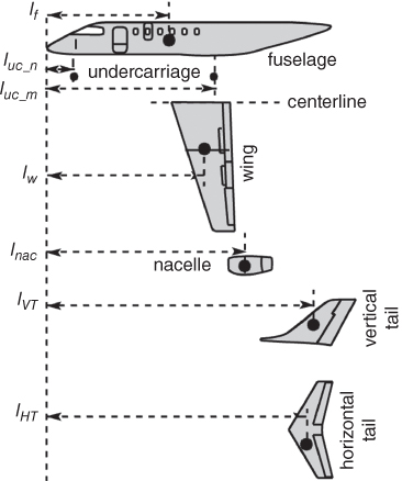
Figure 10.6 Aircraft component CG locations (see Table 10.5).
10.10.13 Fuel – Civil Aircraft
The fuel load is mission specific. For civil aircraft, required fuel is what is needed to meet the design range (i.e. market specification) plus mandatory reserve fuel. It can be determined by the proper performance estimation. At this design stage, statistical data are the only means to estimate fuel load, which is then revised in Chapter 15.
The payload and fuel mass are traded for off‐design ranges; that is, a higher payload (if accommodated) for shorter range and vice versa.
10.11 Centre of Gravity Determination
After obtaining the component masses (i.e. weights), it is now time to locate the aircraft CG. A reference‐coordinate system is essential for locating the CG position relative to an aircraft. A suggested coordinate system is to use the x‐axis along the ground level (or at another suitable level). Typically, the fuselage axis is parallel or nearly parallel to the x‐axis. The z‐axis is orthogonal to x‐axis, passing through the farthest point of the nose cone (i.e. tip), as shown in Figure 10.6. If the x‐axis is taken as fuselage axis then the z‐axis can be the zero reference plane (ZRP).
The first task is to estimate the CG position for each component group from the statistical data. Figure 10.6 provides generic information for locating the positions. Typical ranges of the CG position relative to the component are given in Table 10.5. At this stage, the extreme forward‐most and rearmost CG positions (i.e. x‐coordinates) have not been determined and will be done later.
Table 10.5 Typical values of component CG locations – civil aircraft.
| Component | CG and typical % of component characteristic length | |
| 1. | Fuselage group | 40–45% (military aircraft on higher percentage) |
| 2. | Wing group | No slat – ≈ 30% of MAC |
| With slat ≈ 25% MAC | ||
| 3. | H‐tail group | ≈30% of MACH‐tail |
| 4. | V‐tail group | ≈30% of MACV‐tail |
| 5. | Undercarriage group | At wheel centre as positioned (nose and main wheels taken separately) |
| 6. | Nacelle + pylon group | As positioned (wing or fuselage mount) @ ≈ 40% of nacelle length |
| 7. | Miscellaneous | As positioned – use similarity |
| 8. | Power plant group | As positioned (wing or fuselage mount) @ ≈ 50% of engine length |
| 9. | Systems group | As positioned – use similarity (typically 35–40% of fuselage) |
| 10. | Furnishing group | As positioned – use similarity |
| 11. | Contingencies | As positioned (adjustable to ballast) |
| MEM | (Need not compute for CG at this moment) | |
| 12. | Crew | As positioned |
| OEM | Compute | |
| 13. | Payload | As positioned (distribute around CG) |
| 14. | Fuel | As positioned (distribute around CG) |
| MTOM | Compute | |
| MRM | Compute |
It must be emphasised that the conceptual design phase relies on designers' experience supported by the available statistical data. Aircraft components' CG locates the aircraft CG; therefore, the components must be positioned accordingly. At the conceptual design phase (i.e. not yet manufactured), it is not possible to obtain accurate component weights and their CG locations are yet to evolve. Designers' experience is the way to minimise error. However, errors at this stage do not hinder the progress of the conceptual design, which is revised through iterations for better accuracy. The industry can then confidently predict the accuracy level within ±3 to ±5%, which is sufficient to study the competition before the go‐ahead is given.
Immediately after go‐ahead is obtained, a considerable amount of budget is released for the Project Definition when major structural details are drawn in CAD to obtain a more accurate component weight and the CG location. Also bought‐out items for systems, the undercarriage and power plant are identified and suppliers of these items provide accurate weight and CG data. In fact, during the project definition study, very accurate predictions (less than ±2 to ±3%) can be obtained.
Expressions for ![]() ,
, ![]() and
and ![]() coordinates are given in Eqs. 10.55–10.57
coordinates are given in Eqs. 10.55–10.57
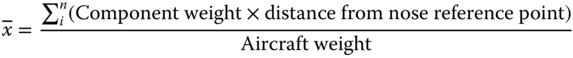

Aircraft weight
If the computation does not indicate the CG within the specified ranges, then move the wing and/or engine(s) to bring CG around the desired percentages of the mean aerodynamic chord (MAC) until a satisfactory solution reached. Moving the wing would also move the CG and neutral point – this may require iteration (wing‐chasing). Fuel tanks can be slightly modified. Batteries are heavy items (or any other heavy items that can be moved) and can be located at a desirable position, that is, fine‐tune the CG location.
10.12 Worked‐Out Example – Bizjet Aircraft
The semi‐empirical relations described in Section 10.10 are now applied to obtain an example of the configuration worked out in Chapters 8 and 9 in the preliminary configuration layout based on guessed MTOM. In this section, more accurate estimates of component and aircraft mass along with the CG locations of the Bizjet aircraft are established. In case there is an unacceptable difference between the guessed and estimated MTOM, then the preliminary Bizjet aircraft configuration needs to be refined through an iterative process with more accurate data. The iteration process may require the repositioning of aircraft components. From Section 8.9, the following are obtained for the preliminary baseline Bizet aircraft configuration.
MTOM = 9500 kg (initially guessed, and to be refined in this exercise).
Two turbofans (i.e. Honeywell TFE731), each with TSLS = 17 235 N (3800 lbs), BPR 4 and dry weight of 379 kg (836 lbs).
The results from this section are compared with the graphical solutions in Figure 10.3 and in Table 10.3.
10.12.1 Fuselage Group Mass
Consider a 5% weight reduction due to composite usage in non‐load‐bearing structures (e.g. floorboards).
Use Eq. 10.19:
For civil aircraft having nult < 0, then (MTOM × nult)x = 1; therefore:
There is a 5% reduction of mass due to use of composites MFcivil = 0.95 × MFcivil_all metal ≈ 930 kg
Checking with Torenbeek's method (Eq. 10.16)
The higher value of the two (930 kg) is kept. This gives a safer approach to begin with.
10.12.2 Wing Group Mass
Consider that it has a 10% composite secondary structure, that is, kmat = (0.9 + 0.9 × 0.1) = 0.99.
It has no slat making ksl = 1.0 and is without a winglet, kwl = 1. For the spoiler, ksl = 1.01 and for a wing‐mounted undercarriage kuc = 1.02. Equation 10.23 gives
where cw = 0.0215 and flaps are standard fitment to the wing.
SW = 30 m2, nult = 4.125, b = 15 m, AR = 6.75, λ = 0.375, Fuel in wing, MWR = 1140 kg, Λ = 14° and t/c = 0.10. Load factor, n = 3.8.
Equation 10.23 becomes:
10.12.3 Empennage Group Mass
Use Eq. 10.25.
Horizontal Tail:
A conventional all moving tail has kemp = 0.2, kconf = 1.0. Consider that it has a 20% composite secondary structure, that is, kmat = (0.8 + 0.9 × 0.2) = 0.98.
MTOM = 9500 kg, nult = 3.8, SHT = 5.5 m2 (exposed), AR = 3.5, λ = 0.3, Λ = 16° and t/c = 0.10.
Use Eq. 10.27.
Vertical Tail (T‐tail):
kconf = 1.5. Consider that it has a 20% composite secondary structure, that is, kmat = (0.8 + 0.9 × 0.2) = 0.98.
MTOM = 9200 kg, nult = 3.8, SVT = 3.5 m2 (exposed), AR = 2.0, λ = 0.5, Λ = 20°, t/c = 0.1 and VD = 380 kt = 703.76 km/h = 195.5 m s−1.
Use Eq. 10.28.
10.12.4 Nacelle Group Mass
The Honeywell TFE731 at dry weight is 379 kg per engine.
Engine thrust = 17 230 N (3800 lb) per engine with a BPR 4.
Use Eq. 10.29: Mnac + pylon = 0.3 × 379 = 113.7 ≈ 114 kg/nacelle
Two nacelles = 228 kg.
10.12.5 Undercarriage Group Mass
MTOM = 9500 kg low‐wing mount; MU/C wing = 0.04 × 9500 = 380 kg.
10.12.6 Miscellaneous Group Mass
Fortunately, there are no miscellaneous structures in the examples considered herein.
10.12.7 Power Plant Group Mass
This is determined from statistics until it is sized in Chapter 14. A typical engine is of the class Allison TFE731–20 turbofan with thrust per engine = 15 570 N to 17 230 N (3500–3800 lbs).
If a manufacturer's dry weight is available, it is better to use it rather than semi‐empirical relations. In this case, the manufacturer's dry weight is in the public domain. MDRYENG = 379 kg per engine. This gives:
The total power plant group mass can be expressed semi‐empirically as
MENG = 1.4 × MDRYENG per engine = 1.4 × 379 = 530.5 kg ≈ 530 kg. For two engines, MENG = 1060 kg.
10.12.8 Systems Group Mass
MTOW = 9500 kg (use Eq. 10.47), MSYS = 0.11 × 9500 = 1045 kg.
10.12.9 Furnishing Group Mass
MTOW = 9500 kg (use Eq. 10.50), MFUR = 0.065 × 9500 = 618 kg.
10.12.10 Contingency and Miscellaneous Group Mass
MTOW = 9500 kg (use Eq. (10.53 and 10.54)), MCONT = 0.016 × 9500 = 152 kg.
10.12.11 Crew Mass
There are two flight crew members and no cabin crew. Therefore, MCREW = 2 × 90 = 180 kg.
10.12.12 Payload Mass
There are 10 passengers. Therefore, MPL = 10 × 100 + 100 = 1100 kg.
10.12.13 Fuel Mass
The range requirement is 2000 nm carrying 10 passengers. From statistical data given in Table 10.1, take the highest value of 26% of MTOW, MFUEL = 0.26 × 9500 = 2470 ≈ 2500 kg.
10.12.14 Weight Summary
Table 10.7, later, is the weight summary obtained by using the coursework example worked out thus far. The last column provides the estimation as a result of the graphical solution (in bracket – kg).
This computation requires further iterations to be fine‐tuned for better accuracy. The CG position is established in the next section, where further iterations will yield a better picture.
Variant Aircraft in the Family
For simplification, linear variations are considered, which should be worked out as a coursework exercise.
Long Variant. Increase payload = 400 kg, fuselage = 300 kg, furnish = 200 kg, fuel = 300 kg and others = 200 kg. Total increase = +1400 kg; MTOMLong = 10 900 kg (no structural changes).
Small Variant. Decrease payload = 500 kg, fuselage = 350 kg, furnish = 250 kg, fuel = 350 kg and others = 250 kg (lightening of the structures). Total decrease = −1700 kg; MTOMSmall = 7800 kg.
10.12.15 Bizjet Aircraft Mass and CG Location Example
The x‐axis is the fuselage axis and ZRP is the y‐axis. Table 10.6 and Eqs. 10.55 and 10.56 are used to locate the CG. SI units are used. Determination of aircraft NP is not done in this book but taken at around 55% of wing MAC.
Table 10.6 Determination of Bizjet CG location.
| Item group | Mass (kg) | X (m) | Moment | Z (m) | Moment |
| Fuselage @ 40% | 930 | 6.08 | 5655 | 1.4 | 1 302 |
| Wing @ 30% of MAC | 854 | 7.4 | 6320 | 1 | 854 |
| H‐tail | 118 | 14 | 1652 | 8 | 944 |
| V‐tail | 83 | 15 | 1245 | 3 | 249 |
| Undercarriage (nose) | 110 | 1.8 | 198 | 0.4 | 44 |
| Undercarriage (main) | 270 | 8 | 1840 | 0.5 | 135 |
| Nacelle/pylon | 228 | 10.5 | 2415 | 2 | 460 |
| Miscellaneous | |||||
| Power plant | 1060 | 10.7 | 11 342 | 2 | 2120 |
| Systems | 1045 | 6.5 | 6793 | 1 | 1045 |
| Furnishing | 618 | 6 | 3708 | 2 | 1236 |
| Contingencies | 152 | 3 | 456 | 1.2 | 182 |
| MEM | 5470 | ||||
| Crew | 180 | 3 | 540 | 1.4 | 252 |
| Consumable | 120 | 4 | 480 | 1.5 | 180 |
| OEM | 5770 | ||||
| Payload | 1100a | 6.2 (6.4) | 7040 | 1.1 | 1210 |
| Fuel | 2500 | 7.8 | 19 500 | 1 | 2500 |
| Total moment at MTOM of 9370 ≈ 9400 | 69 184 | 12 713 | |||
| MRM | 9450 | ||||
Bold values highlight the most important parameters.
aNo frills 10 passengers or a luxury arrangement for eight passengers.
The CG should lie in the plane of symmetry (there are unsymmetrical aircraft).
The CG locations for the CGLong Variant and the CGShort Variant may be worked out by the readers.
10.12.16 First Iteration to Fine‐Tune CG Position Relative to an Aircraft and Components
The preliminary aircraft configuration begins in Chapter 8 with a guesstimated MTOM, engine size and CG position. It is unlikely that the computed aircraft mass as worked out in this chapter will match the estimated mass. In fact, the example shows that it is lighter, with a more accurate CG position; therefore, this replaces the estimated values in Chapter 8. The differences from guesstimate and revised in chapter are as follows.
Also note that both mass and CG location are slightly different from preliminary data.
| Estimated at concept definition | Revised in Chapter 9 (Figure 9.22) | |
| (Chapter 8) | First iteration in Chapter 10 | |
| MTOM – kg | 9500 | 9400 |
| MAC leading edge location – m from ZRP | 6.77 | 6.76 |
| Aft CG limit, |
7.4 m | 7.36 m |
| CG position, |
1.38 m | 1.352 m |
The differences are small. From now onwards, the revised values will used; most importantly the MTOM is now revised to 9400 kg. In principle, the aircraft configuration must be revised at this stage of progress as the first iteration. The worked‐out example of the Bizjet shows small differences, hence no iteration is carried out as a simple repositioning of battery, black‐boxes and so on will do the job. In that case the angle, β, is kept satisfied. Final sizing is accomplished in Chapter 14, when iteration may be required.
MILITARY AIRCRAFT
10.13 Mass Fraction Method – Military Aircraft
National defence requirements made military designs evolve rapidly, incorporating new technologies at a considerable cost to stay ahead of potential adversary. Whereas miniaturisation of electronic and other equipment reduces onboard mass, increased demand in combat capabilities worked in the opposite direction to add mass. Combat aircraft size kept growing to exceed 35 000 kg for multirole fighter aircraft. Earlier, it was holding on at around 16 000 kg. With improved missile capabilities, aircraft performance demand is now somewhat changed, especially in reaching maximum speed. Combat aircraft takeoff mass varies according to mission requirement. The Typical Takeoff Mass (TTOM) is less than MTOM. It is beneficial to have a small lightweight fighter, but currently with less than 12 000 kg of MTOM, armament capacity and radius of action would suffer in a demanding mission. Light combat aircraft has to be seen to cater mainly for high‐subsonic/low supersonic combat missions, unlikely to exceed Mach 1.4. The following points are pertinent to military aircraft component mass estimation methodologies.
- Combat aircraft (fighters) have engines buried in the fuselage; hence, there is no wing relief benefit.
- A combat role has a wide spectrum of activities, as outlined in Section 4.12. In general, close support/ground attack aircraft (no afterburning engines) are subsonic with quick turning capabilities, whereas air superiority aircraft have supersonic capabilities with afterburning turbofans.
- Modern supersonic combat aircraft configurations show considerable wing‐body blending.
- Dominantly, all expendable payload is externally mounted except for bigger designs, which could have internal bomb load. Modern military aircraft have an external load that is contoured and flushed with mouldlines. Internally mounted guns are permanent fixtures, integral to the airframe structure. Training military aircraft pylons to carry external load are not taken as permanent fixtures.
- Consumables (e.g. firing rounds) are internally loaded. In general, for long‐range missions, there is than one crew and some consumables meant for them.
Military designs are technology specific and, as a result, unlike civil design, military designs exhibit large variations in statistical distribution.
Generic military aircraft component mass is listed in MIL‐STD‐1374 in exhaustive detail, which is not required in the conceptual design stage. As with civil aircraft design, this section presents a consolidated generalised group for what is required at the conceptual design phase. Note that military aircraft do not have cabin crew and passengers. The payload is weaponry and is mostly carried externally. Section 10.6 gives the military aircraft component nomenclature.
Table 10.7 Military aircraft mass fraction (see Section 10.6.1 for symbols).
| Group | Trainer | Combat (all turbofan) | |||
| Turboprop | Turbofan | Close support fighter | Bomber | ||
| Fuselage | Ffu = MF/MTOM | 10–12 | 9–11 | 8–10 | |
| Wing | Fw = Mw/MTOM | 7–9 | 11–14 | 7–10 | |
| H‐Tail | Fht = Mht/MTOM | 1.4–1.8 | 1.2–1.6 | 1–1.5 | |
| V‐Tail | Fvt = Mvt/MTOM | 0.7–0.9 | 0.8 | 0.7–1 | |
| Intake | Fin = Min/MTOM | 0.8–1.2 | 1–1.2 | 1.5–2 | |
| Pylon (weapon) | Fpy = Mpy/MTOM | 0.3–0.5 | 0.2–0.4 | 0.2–0.3 | |
| Undercarriage | Fuc = Muc/MTOM | 3–5 | 5–7 | 2.5–4 | |
| Fixed armament | Farm = Marm/MTOM | 1–1.2 | 1–1.2 | 1–1.2 | |
| Engine | Feng = Meng/MTOM | 9–11 | 11–12 | 8–12 | |
| Retarding device | Ftr = Mtr/MTOM | 0 | 0.4–0.6 | 0.5–0.8 | |
| Engine con. | Fec = Mec/MTOM | 0.5–0.8 | 1–1.6 | 0.7–0.9 | |
| Fuel sys. | Ffs = Mfs/MTOM | 0.5–0.6 | 2–3 | 2–3 | |
| Oil sys. | Fos = Mos/MTOM | 0.2–0.4 | 0.2–0.4 | 0.3–0.4 | |
| Flight con. sys | Ffc = Mfc/MTOM | 2–2.5 | 2–2.5 | 1.5–2 | |
| Hydr/pneumatic sys | Fhp = Mhp/MTOM | 0.5–0.8 | 0.5–0.8 | 0.8–1 | |
| Electrical | Felc = Melc/MTOM | 2–2.5 | 1.5–2 | 1–1.4 | |
| Instrument | Fins = Mins/MTOM | 0.6–1 | 0.4–0.5 | 0.5–0.6 | |
| Avionics | Fav = Mav/MTOM | 3–4 | 3–6 | 4–6 | |
| ECS + oxygen | Fecs = Mecs/MTOM | 0.6–1 | 0.5–0.8 | 1–1.2 | |
| Seat + escape sys | Ffur = Mfur/MTOM | 1.2–1.5 | 1–1.4 | 1–1.4 | |
| Misc. | Fmsc = Mmsc/MTOM | 0 | 1 | 1 | |
| Paint | Fpn = Mpn/MTOM | 0.01 | 0.01 | 0.01 | |
| Contingency | Fcon = Mcon/MTOM | 1 | 1 | 1 | |
| MEW – % | 52–56 | 58–64 | 49–53 | ||
| Crew | 5–6 | 0.8–1.2 | 0.8–1 | ||
| Consumable | 0 | 0 | 0 | ||
| OEW – % | 57–60 | 60–65 | 50–54 | ||
| Payload and fuel are traded | |||||
| Payload | 15–25 | 15–20 | 20–25 | ||
| Fuel | 15–20 | 18–20 | 20–25 | ||
| MTOM – % | 100 | 100 | 100 | ||
Military aircraft follow the same procedure for mass fraction estimation method as that of civil aircraft but have a different mass fraction (shown in percentage) of Mi/MTOM, where subscript ‘i’ represents the ith component. All items should total 100% of the MTOM; this also can be expressed in terms of mass per wing area (i.e. component wing loading). Unlike civil aircraft, each generation of military aircraft takes a bigger leap towards advanced technology driven by the requirements of national security more than profit. Reference [9] gives an exhaustive list of weight breakdown for many relatively older military aircraft designs. A new design should show improvements, especially of newer technologies (e.g. new materials, lighter systems). Table 10.7 (combat and trainer aircraft) gives ballpark figures of mass fraction (in percentages) for arriving quickly at a starting point for the initial configuration obtained in Chapter 6. This time, a wider variation of ±15% (may exceed in a few designs) may be allowed to accommodate a wide range of variation.
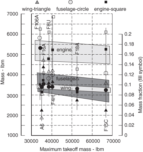
Figure 10.7 Military aircraft fuselage mass.
Note that the OEM fraction in the table agrees with the trend of actual aircraft data shown in Figure 10.8. Lighter aircraft would show a higher mass fraction. A fuselage‐mounted undercarriage is shorter and lighter for the same MTOM. These tables give some idea of component masses at an early project stage. It is best to use more accurate semi‐empirical relations (Section 10.15) to obtain component masses at the conceptual phase. These tables would prove useful to estimate masses (e.g. fuel mass, engine mass etc.) required as a starting point for some semi‐empirical relations.
Discussions in Section 10.8.1 on using the mass fraction method mention it is also valid for military aircraft mass estimation.
10.14 Graphical Method to Predict Aircraft Component Weight – Military Aircraft
In addition to the statistical data on military aircraft given in Section 7.10, this section extends statistical data on military aircraft component mass in graphical form, as illustrated in the following figures.

Figure 10.8 Military aircraft wing mass.
Not much graphical statistical data on military aircraft component mass is available in the public domain. References 9, 10 are a good source of military aircraft component masses. Note that graphs are in the FPS system. As expected, they show wide variation, yet there is a trend through linear regression. Figures 10.7 and 10.8 give the component weights graphs. They show wide dispersion.
10.15 Semi‐Empirical Equations Method (Statistical) – Military Aircraft
The semi‐empirical relations given in this section are meant for high‐subsonic military aircraft mass estimation, for example, light combat aircraft, trainer, close air support (CAS), counter insurgency (COIN) roles and so on. (The reader may refer to 9, 10 for supersonic combat aircraft semi‐empirical relations.) The semi‐empirical relations are derived from theoretical formulation and have been refined with statistical data. The section is divided into subsections, each with a step‐by‐step discussion of workflow.
In a similar manner to civil aircraft, military aircraft have their own sets of semi‐empirical relations derived from theoretical formulation and refined with statistical data. As in the civil mass estimation, there are several forms of semi‐empirical weight prediction formulae proposed by various analysts, all based on the key drivers with refinements as perceived by the proposer. They are similar in nature and yield close enough results. References 1–6, 9, 11 offer more information on weight prediction. The following subsections provide aircraft component weight (mass) semi‐empirical formulae, component‐by‐component.
10.15.1 Military Aircraft Fuselage Group (SI System)
Military aircraft do not have a constant section fuselage and are more densely packed. A combat aircraft fuselage is not pressurised (only cockpit is). In a blended body it is not easy to lineate fuselage line from the wing. The best would be construction specific where the joining line of the wing is the line for fuselage. It is much simpler for the example of the Advanced Jet Trainer (AJT) in hand. In this case take Dave = average of the shape (see Figure 8.14) around the engine. The expression includes fuselage‐mounted side/chin intakes. (The AJT does not have a pod – intake weight is taken as integral with fuselage weight.)
where cfus = 0.175
- kuc = 1.05 for a fuselage‐mounted undercarriage with bulge and 1.03 without bulge.
- kmat = 1.0 for metal, otherwise make a percentage weight reduction.
- kpara = 1.002 if there is a brake parachute, otherwise 1.
- kintake = 1.005
10.15.2 Military Aircraft Wing Mass (SI System)
The equation is simplified by the authors for classroom usage. The same remarks as made for civil aircraft are also applicable to the military case, except that the values of factors change. Military wings are thinner. In many cases, the wing does not carry fuel (e.g. F104) and does not have winglets.
Writing the modified equation in terms of the book's notation, Eq. 10.21 is changed to:
- cw = 0.0215 for AR < 5 (high subsonic – jet)
- = 0.023 for AR > 5 (low subsonic – propeller)
- kmat = effect of material change as in the case of the fuselage
- kuc = 1.002 for a wing‐mounted undercarriage, otherwise 1.0
- ksl = 1.004 for use of a slat and ksp = 1.005 for a spoiler. Flaps are standard.
10.15.3 Aircraft Empennage
The equation is simplified by the authors for classroom usage. The same remarks as made for civil aircraft are also applicable to the military case, except that the values of factors change as follows. Equation 10.25 for civil aircraft gives:
kmat = Effect of material change as in the case of fuselage.
The modified equations, in terms of the notations in Eq. 10.25, are as follows.
Horizontal Tail:
For all tail movement, use kemp = 0.018, kconf = 1.05, otherwise 1.0.
Vertical Tail:
For tail configurations, use kemp = 0.022, kconf = 1.1 for T‐tail, 1.05 for mid‐tail and 1.0 for low tail.
10.15.4 Nacelle Mass Example – Military Aircraft
A typical combat aircraft does not have a nacelle and a pod – intake weight is taken to be integral with fuselage weight.
10.15.5 Power Plant Group Mass Example – Military Aircraft
From the engine TSLS the engine dry mass can be obtained from its thrust‐to‐weight ratio, this typically varies from 5 to 8. It is always better to use engine manufacturer's supplied data that is freely available in the public domain. Otherwise, refer to Table 10.8 to obtain engine dry mass.
Table 10.8 Typical values of component CG locations – military aircraft.
| Component | Military AJT aircraft | |
| Typical % of component characteristic length | ||
| 1. | Fuselage group | 45–50% |
| 2. | Wing group | No slat – 30% of MAC |
| With slat – 25% MAC | ||
| 3. | H‐tail group | 30% |
| 4. | V‐tail group | 30% |
| 5. | Undercarriage group | At wheel centre |
| 6. | Nacelle + pylon group | Generally not applicable |
| 7. | Miscellaneous | As position – use similarity |
| 8. | Power plant group | 70–80% |
| 9. | Systems group | As position – use similarity (typically 35% of fuselage) |
| 10. | Furnishing group | As position – use similarity |
| 11. | Contingencies | As position – use similarity |
| MEM | Compute | |
| 12. | Crew | As position – use similarity |
| OEM | Compute | |
| 13. | Payload | As position – use similarity |
| 14. | Fuel | As position – use similarity |
| MTOM and MRM | Compute | |
For the variant engine mass, only add the increment/decrement of the dry engine mass to the baseline power plant group mass.
The total power plant group mass can be expressed semi‐empirically as
Jet engine
Turboprop
Civil aircraft power plant:
where 1.5 ≤ ktp ≤ 1.8. (due to propeller and intake)
APU (if any)
10.15.6 Undercarriage Mass Example – Military Aircraft
Undercarriage size depends on an aircraft's MTOM. A military aircraft undercarriage is heavier in order to withstand hard landings.
Tricycle type (retractable) – wing‐mounted (nose and main gear estimated together)
For a low‐wing‐mounted undercarriage:
For a mid‐wing‐mounted undercarriage:
For a high‐wing‐mounted have fuselage‐mounted :
For a fixed undercarriage, the mass is 10–15% lighter; for a tail‐dragger, it is 20–25% lighter.
10.15.7 System Mass – Military Aircraft (Higher Mass Fraction for Lighter Aircraft)
System mass comprises of avionics, electrical, plumbing, ECS (oxygen system) and so on.
10.15.8 Aircraft Furnishing (Ejection Seat) – Military Aircraft
As such, military aircraft do not have furnishings but the following can be added:
10.15.9 Miscellaneous Group (MMISC) – Military Aircraft
Carefully examine what structural parts are left out, for example, delta fin and so on. If any item does not fit into the standard groups as listed here – include it in this group. Typically, this be expressed as
10.15.10 Contingency (MCONT) – Military Aircraft
A good designer keeps provision for contingency, that is,
10.15.11 Crew Mass
There are trainer and trainee pilots. Take a mass of 90 kg per crew member.
10.15.12 Fuel (MFUEL)
Fuel load is mission specific. This can be determined by proper performance estimation shown in Chapters 11 and 13. At this stage, statistical data is the only means to guesstimate fuel load that will be revised in Chapters 11 and 13.
Military aircraft is mission specific and also has to depend on statistical data at this stage of design until accurate fuel load can be estimated through performance estimation.
10.15.13 Payload (MPL)
Military aircraft payload is the armament specified by the user requirements. Internal guns are taken as systems weight.
10.16 CG Determination – Military Aircraft
Table 10.8 gives the CG positions of aircraft components of the classroom examples:
x, y and z are measured from the nose of the aircraft and then convert to MACw.
Table 10.8 may be used to determine the CG location. Coordinate origin x = 0 at the nose tip, and z = 0 at ground level, which is kept horizontal.
Equations 10.54–10.56 are valid to compute CG coordinates. See Section 10.12.1 for the classroom Bizjet example to compute ![]() and
and ![]() . The important ‘potato’ curve for CG variation for all loading conditions is left out.
. The important ‘potato’ curve for CG variation for all loading conditions is left out.
The readers should make sure that it has the static margin with full crew. The CG should be at around 18% of MAC when fully loaded and at around 22% when empty, only in between with pilots. CG is always forward of the NP. (Where is it? Take 50% of the MAC.) This is for static stability reasons.
If the computation does not indicate the CG within the specified ranges, then move the wing and/or engine to bring the CG to the desired percentages of the MAC until a satisfactory solution is reached. Fuel tanks can be slightly modified. Batteries are heavy items and can be located at a desirable position to fine‐tune the CG location to the desired position.
10.17 Classroom Example of Military AJT/CAS Aircraft Mass Estimation
The user requirement for practice bombs and missiles is 1800 kg, this is a reasonable practise armament load. Therefore, MPL = 1800 kg. The fully loaded AJT is estimated to be 6500 kg (Figure 8.12). AJT structure is designed to cater for: MTOM = 6600 kg, wing area SW = 17 m2.
CAS structure will have MEM to withstand the maximum MTOM, but the MEM does not change as is explained next for the incremental mass required to beef up the structure. The structural component commonality can be maintained by beefing up the main load‐bearing members of a structure. To the undercarriage is to maintain component commonality without any modification, hence it is sized to CAS MTOM of 7500 kg. CAS armament payload is 2300 kg.
Only the shorter CAS nose cone replaces the longer AJT nose cone as one pilot is removed (Figure 8.14). In summary, both the variants will have same MEM.
AJT manoeuvre limits are as follows.
- Manoeuvre limits: +7 g to −3.5 g for the training mission without armament at 4800 kg
- Manoeuvre limits: +6 g to −3 g for the armament training mission at 6600 kg
CAS manoeuvre limits are as follows.
- Manoeuvre limits: +8 g to −4 g for the TTOM (lower fuel and armament) @ 7000 kg
- Manoeuvre limits: +7 g to −3.5 g for the MTOM @ 7500 kg
The never‐exceed speed, VD = 620 kn (0.95 Mach).
10.17.1 AJT Fuselage (Based on CAS Variant)
Consider that it has a 10% weight saving on account of composite usage in secondary structures (10%), that is, kmat = 0.99. MTOM = 6500 kg. L = 12.1 m, Dave = 0.5 × (1.8 + 0.9) = 1.35 m and VD = 620 kt = 1150 km/h = 319.4 m s−1, nult = 6 g. Equation gives:
10.17.2 AJT Wing (Based on CAS Variant)
Consider that it has a 10% weight saving on account of composite usage in secondary structures (10%), that is, kmat = 0.99. MTOM = 6500 kg. nult = 6 g, SW = 17 m2, AR = 5.3, λ = 0.3, MWR = 828 kg, Λ = 20°, t/c = 0.10 and = 1150 km/h = 319.4 m s−1. It has no slat making ksl = 1 and has 828 kg fuel in the wing. For the spoiler, ksl = 1.005 and the undercarriage is not wing‐mounted kuc = 1. Equation gives:
10.17.3 AJT Empennage (Based on CAS Variant)
Horizontal Tail: Equation gives:
Consider that it has a 10% weight saving on account of composite usage in secondary structures (10%), that is, kmat = 0.99. MTOM = 6500 kg.
AJT horizontal tail is all moving, that is, configuration factor kconf = 1.05. Note that the exposed area constitutes as the empennage mass as constructed.
Vertical Tail: Equation gives:
10.17.4 AJT Nacelle Mass (Based on CAS Variant)
The AJT does not have a pod – the intake weight is taken to be integral to the fuselage weight.
10.17.5 AJT Power Plant Group Mass (Based on AJT Variant)
Suitable engines in the class are the following. Both have BPR = 0.75 and engine = 22 in.
For AJT – Adour 861 producing 26.66KN (6000 lb), dry weight = 590 kg (1300 lb).
For CAS – Adour 871 producing 31.4KN (7060 lb), dry weight = 610 kg (1330 lb).
Taking Adour 871 for AJT (weights will not change with final engine sizing in Chapter 14).
Total power plant group mass can be expressed semi‐empirically as (Eq. gives):
10.17.6 AJT Undercarriage Mass (Based on CAS Variant)
To maintain commonality, use the heaviest fully loaded CAS mass of 7500 kg. This is the only time CAS maximum mass has been applied to get component mass.
For fuselage‐mounted undercarriage use Eq. 10.68.
10.17.7 AJT Systems Group Mass (Based on AJT Variant)
Equation 10.65 gives:
10.17.8 AJT Furnishing Group Mass
Ejection seat plus the oxygen system are taken in this group to be 90 kg per crew member.
10.17.9 AJT Contingency Group Mass
Equation 10.71 gives:
10.17.10 AJT Crew Mass
There are trainer and trainee pilots. Therefore, MCREW = 2 × 90 = 180 kg
10.17.11 AJT Fuel Mass (MFUEL)
Fuel load is mission specific. From AJT statistics in Section 6.12.1, MFUEL_NTC = MNFC − OEW = 4800–3700 = 1100 kg (tank not full).
It is assumed that practise range is less than 100 miles away and an AJT reaches the range at economic cruise to make two to three passes for armament training at a sortie duration of about 50 minutes. The tankage capacity can hold 1400 kg fuel for ferry flights and, if required, an AJT armament practice sortie can be made longer at a slightly higher MTOM.
10.17.12 AJT Payload Mass (MPL)
Military aircraft payload is its armament, which is specified by the user requirements. Internal guns are taken as systems weight. Practice armament (includes gun ammunition) = 1800 kg.
10.18 AJT Mass Estimation and CG Location
Use Table 10.5 and Eqs. 10.40 and 10.41 to locate CG location. SI units (kg and m) are used.
Table 10.9 gives the CG locations of aircraft components of the classroom examples:
Table 10.9 Typical values of component CG locations – AJT.
| Item group | Mass (kg) | X (m) | Moment | Z (m) | Moment |
| Fuselage | 882 | 6.6 | 5821 | 1.3 | 1164 |
| Wing | 466 | 7.2 | 3355 | 1.75 | 816 822 |
| H‐tail | 91 | 11.31 | 1029 | 1.9 | 173 |
| V‐tail | 42 | 10.66 | 448 | 2.4 | 100 |
| Undercarriage (nose) | 80 | 2.0 | 160 | 0.48 | 36 |
| Undercarriage (main) | 220 | 7.4 | 1628 | 0.5 | 110 |
| Nacelle + pylon | None | ||||
| Miscellaneous | None | ||||
| Power plant | 724 | 8.6 | 6226 | 1.32 | 956 |
| Systems | 650 | 5.2 | 3380 | 1.2 | 780 936 |
| Ejection seats | 180 | 4 | 720 | 1.32 | 237 |
| Contingencies | 65 | 4 | 392 | 1.32 | 87 |
| MEM | 3400 | ||||
| Crew | 180 | 4 | 720 | 1.32 | 237 |
| OEM | 3580 | ||||
| Fuel (wing and fuselage) | 1100 | 7.8 | 8580 | 1.65 | 1815 |
| Total NTC mass | 4680 ≈ 4800 | 32 459 | 6459 | ||
| CG at NTC mass | |||||
| Armament payload | 1800 | 6.6 | 11 880 | 1.4 | 2520 |
| Total MTOM | 6 80 ≈ 6500 | 44 339 | 8979 | ||
| CG at MTOM |
Bold values highlight the most important parameters.
The CG location is very close to what was guessed in Section 9.16.2 hence avoided iterations. The angle, β, for NTC and MTOM has also been estimated in Section 9.16.2, within the acceptable range. Readers may compute the CAS CG location. Proper CG positioning can be established after aircraft NP is established when the forward and aft CG limits can be ascertained by fine‐tuning component positions. Determination of aircraft NP is not done in this book but taken at around 40% of wing MAC.
The angle, β, for NTC and MTOM has been estimated also in Section 9.16.2, within the acceptable range. This is a satisfactory angle covering maximum fuselage‐rotation angle at takeoff.
The external geometry being the same, the CAS variant can be extrapolated from the AJT variant to a fair degree accuracy as reasoned here.
- The OEM for both the variants stays about the same as the removal of the masses of one crew, plus the ejection seat and mass saving from a slightly shorter fuselage (see Figure 8.14) are taken up as structural reinforcements to support a higher MTOM, manoeuvring load and avionic upgrade. This amounts to 220 kg.
- Fuel load increment, ΔFuel = 300 kg (to full tank capacity, armament load increment, ΔPayload = 500 kg, avionics and systems mass increment, ΔSystems (small radar) = 80 kg, bigger engine power plant mass increment, ΔPowerplant = 20 kg. This totals a mass increment, ΔMTOM = 900 kg. Therefore, CAS MTOM is expected to be around 7500 kg. The figures would be iterated as more information is generated. The aim is to make new design better than any existing aircraft in the class. This is where the experience of designers counts.
The preliminary aircraft configuration begins in Chapter 8 with a guesstimated MTOM, engine size and CG position. It is unlikely that the computed aircraft mass as worked out in this chapter will match the estimated mass. In fact, the example shows that it is lighter, with a more accurate CG position; therefore, this replaces the estimated values in Chapter 8. The differences from guesstimate and revised in chapter are as follows.
| Guessed at concept definition (Chapter 8) |
Revised in Chapter 9 (Figure 9.23) First iteration in Chapter 10 |
|
| MTOM – kg | 6500 | 6500 |
| CG position, |
1.35 m | 1.345 m |
| CAS variant MTOM – kg | 7500 | 7400 |
Exact MTOM agreement is, in a way, coincidental, although statistics in Figure 8.12 indicate what is to be expected. The differences in CG locations are small and the revised values are taken as its iteration. In principle, the aircraft configuration must be revised at this stage of progress as the first iteration. Final sizing is accomplished in Chapter 14, when iteration is required. Coursework may require only one iteration cycle of computation.
10.19 Classroom Example of a Turboprop Trainer (TPT) Aircraft and COIN Variant Weight Estimation
The user requirement for practice bombs and missiles is 500 kg, this is a reasonable practise armament load. Therefore, MPL = 1800 kg. The fully loaded TPT is estimated to be 2800 kg (Figure 10.9).
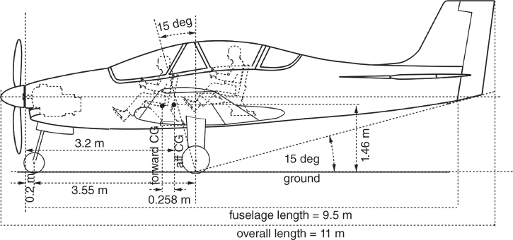
Figure 10.9 Turboprop trainer aircraft (TPT).
Manoeuvre: +7 g to −3.5 g for the trainer version at NTCM (Normal Training Configuration Mass) without practise armament (fully aerobatic)
Manoeuvre: +6 g to −3 g for fully armed version at MTOM
The following are the TPT details estimated as the concept definition from the statistical data that will be finalised to the formal sized configuration in Chapter 16.
| MTOM = 2800 kg (6160 lbm) | NTC‐TOM = 2350 kg (5170 lbm) |
| OEW = 1700 kg (3740 lbm) | |
| Crew = 180 kg (396 lbm) | Fuel = 500 kg (110 lbm) |
| Maximum speed = 280 kt | Sustained speed = 240 kt (405.2 ft s−1) |
| MTOM = 2800 kg (6160 lb) | NTCM = 2350 kg (5170 lb – no armament) |
| OEW = 1700 kg (3740 lb) | Practise armament load = 450 kg (≈1000 lb) |
| Crew = 400 lb (≈180 kg) | Fuel = 470 kg (1012 lb/kg) |
| Typical mid‐training aircraft mass = 2200 kg (4840 lb) | |
| Maximum speed = 280 kt | Sustained speed = 240 kt (405.2 ft s−1) |
Fuselage
| Length = 9.5 m (31.16 ft) | height = 1.6 m (5.25 ft) | |
| Cockpit width = 0.88 m (35 in) | Fuselage width = 1.0 m (≈40 in) | |
| Fineness ratio = 9.5/1.0 = 9.5 | ||
| Wing (Wing Aerofoil): National Advisory Committee for Aeronautics (NACA) 632‐215) | ||
| Reference area = 16.5 m2 (177.3 ft2) | Span = 16.36 m (53.8 ft) | AR = 6.5 |
| Root chord, CR = 2.36 m (7.74 ft) | Tip chord, CT = 0.82 m (3.7 ft) | |
| MAC = 1.715 m (5.62 ft) | Taper ratio, λ = 0.35 | Λ¼ = 0° |
| Dihedral = 5° (dihedral – low wing) | Twist = 1° (wash out), | t/c = as specified |
| Flap = 2.2 m2 (23.6 ft2) | Aileron = 1.06 m2 (11.4 ft2) |
H‐tail (NACA 0012)
| Reference area = 4.1 m2 (44.2 ft2) | Span = 4.2 m (13.8 ft) | Aspect ratio = 4.0 |
| Root chord, CR = 1.28 m (4.2 ft) | Tip chord, CT = 0.67 m (2.2 ft) | |
| H‐tail MAC = 1 m (3.3 ft) | Taper ratio, λ = 05, Λ¼ = 0° | |
| Elevator area = 1.025 m2 (11 ft2) | t/c = 0.12 |
V‐tail (NACA 0012)
| Reference area = 2.2 m2 (23.3 ft2) | Height = 1.375 m (4.52 ft) |
| Root chord, CR = 1.64 m (5.38 ft) | Tip chord, CT = 0.66 m (2.16 ft) |
| V‐tail MAC = 1.28 m (4.2 ft) | Taper ratio, λ = 04, Λ¼ = 20° |
| Rudder area = 0.44 m2 (4.74 t2) | t/c = 0.12 |
Engine
| Takeoff static power at International Standard Atmosphere (ISA) sea level = 975 shp | (Garratt TPT‐331‐12B) |
| Dry weight = 182 kg (400 lb), | Engine intake area = 0.048 m2 (0.52 ft2) |
| Length = 1.1 m (43.4 in) | Height = 0.686 m (27 in.) |
COIN Variant
A COIN variant can be derived, affecting the external geometry, by re‐engineering the trainer version with 1200 SHP turboprop, increasing armament load to 1000 kg by adding Δ550 kg of combat weapons, increasing fuel capacity to 1000 kg by adding Δ570 kg of fuel that will require adding strength to structure with OEM raised by about Δ400 kg to nearly 3000 kg MTOM. This is merely a suggestion and is not worked out. The readers may give this a try.
10.19.1 TPT Fuselage Example
Consider that it has a 10% weight saving on account of composite usage in secondary structures (10%), that is, kmat = 0.99. MTOM = 2800 kg. L = 9.5 m, Dave = 0.5 × (1.8 + 0.9) = 1.35 m and VD = 300 kt = 556.5 mph = 155 m s−1, nult = 6 g. Equation 10.58 gives:
10.19.2 TPT Wing Example
Consider that it has a 10% weight saving on account of composite usage in secondary structures (10%), that is, kmat = 0.99. MTOM = 2800 kg. nult = 6 g, SW = 16.5 m2, AR = 6.5, λ = 0.5, Λ = 0°, t/c = 0.15 and = 280 kt = 144 m s−1. It has no slat making ksl = 1.0, kuc = 1.002 and has 470 kg fuel in the wing. For the spoiler, ksl = 1.005 and the undercarriage is not wing‐mounted kuc = 1. Equation 10.59 gives:
10.19.3 TPT Empennage Example
Horizontal Tail:
Equation 10.60 gives:
Consider that it has a 10% weight saving on account of composite usage in secondary structures (10%), that is, kmat = 0.99. MTOM = 6600 kg.
AJT horizontal tail is all‐moving, that is, configuration factor kconf = 1.05. Note that the exposed area constitutes as the empennage mass as constructed.
Vertical Tail: Equation 10.61 gives:
10.19.4 TPT Nacelle Mass Example
The TPT does not have a pod‐intake weight taken to be integral with fuselage weight.
10.19.5 TPT Power Plant Group Mass Example
Use Eq. 10.62:
Engine selected is Garratt TPT‐331‐12B (include propeller) derated to 1000 SHP.
For TPT – Garratt TPT‐331‐12B, dry weight = 175 kg (385 lb).
For COIN – Garratt TPT‐331‐12B at the rated power of 1100 SHP.
10.19.6 TPT Undercarriage Mass Example (Based on CAS Variant)
To maintain commonality, use the heaviest fully loaded COIN mass of 3100 kg. This is the only time COIN maximum mass has been applied to get component mass.
For a fuselage‐mounted undercarriage use Eq. 10.65.
10.19.7 TPT Systems Group Mass Example
Use Eq. 10.68
MTOW = 2800 kg, MSYS = 0.12 × 2800 = 336 kg.
10.19.8 TPT Furnishing Group Mass Example
Ejection seat plus oxygen system are taken in this group to be 80 kg per crew member.
10.19.9 TPT Contingency Group Mass Example
Use Eq. 10.71:
MCONT = 0 for TPT.
10.19.10 TPT Crew Mass Example
There are trainer and trainee pilots. Therefore, MCREW = 2 × 90 = 180 kg.
10.19.11 TPT Fuel (MFUEL)
Fuel load is mission specific. The tankage capacity can hold 1000 kg fuel.
10.19.12 TPT Payload (MPL)
Military aircraft payload is its armament, which is specified by the user requirements. Internal guns are taken as systems weight. Practice armament (includes gun ammunition) = 1800 kg.
10.20 Classroom Worked‐Out TPT Mass Estimation and CG Location
Use Table 10.5 and Eqs. 10.40 and 10.41 to locate CG location. SI units (kg and m) are used.
Table 10.10 gives the CG locations of aircraft components of the classroom examples:
Table 10.10 Typical values of component CG locations – TPT.
| Item group | Mass (kg) | X (m) | Moment | Z (m) | Moment | |
| Fuselage | 358 | 3.8 | 1360 | 1.45 | 519 | |
| Wing | 282 | 3.75 | 1057 | 1.2 | 338 | |
| H‐tail | 63 | 9.15 | 576 | 2.0 | 126 | |
| V‐tail | 24 | 9.55 | 229 | 2.85 | 68 | |
| Undercarriage (nose) | 35 | 0.22 | 6.6 | 0.35 | 11 | |
| Undercarriage (main) | 100 | 3.75 | 338 | 0.36 | 32 | |
| Miscellaneous | None | |||||
| Power plant | 327 | 0.4 | 131 | 1.6 | 523 | |
| Systems | 336 | 1.7 | 714 | 1.3 | 546 | |
| Ejection seats | 180 | 3.7 | 666 | 1.55 | 279 | |
| Contingencies | 0 | 5.4 | 140 | 1.4 | 36 | |
| MEM | 1688 ≈ 1700 | |||||
| Crew | 180 | 3.7 | 666 | 1.6 | 288 | |
| OEM | 1880 ≈ 1900 | |||||
| Fuel (wing and fuselage) | 450 | 3.8 | 1710 | 1.8 | 2.0 | 810 |
| Total NTC mass | 2350 | 7595 | 3576 | |||
| CG at NTC mass | ||||||
| Armament payload | 450 | 3.6 | 1800 | 1.4 | 7000 | |
| Total MTOM | 2800 | 9585 | 4484 | |||
| CG at MTOM | ||||||
Bold values highlight the most important parameters.
The CG location is very close to what was estimated in Section 9.16.2, hence iterations were avoided. The angle, β, for NTC and MTOM has also been estimated in Section 9.16.2, within the acceptable range. Readers may compute the CAS CG location. Proper CG positioning can be established after aircraft NP is established when the forward and aft CG limits can be ascertained by fine‐tuning component positions. Determination of aircraft NP is not done in the book but taken to be at around 40% of wing MAC.
This is a satisfactory angle covering maximum fuselage‐rotation angle at takeoff.
The preliminary aircraft configuration begins in Chapter 8 with a guesstimated MTOM, engine size and CG position. It is unlikely that the computed aircraft mass as worked out in this chapter will match the estimated mass. In fact, the example shows that it is lighter, with a more accurate CG position; therefore, this replaces the estimated values in Chapter 8. The differences from guesstimate and revised in chapter are as follows.
| Guessed at concept definition | Revised in Chapter 9 (Figure 9.24) | |
| (Chapter 8) | First iteration in Chapter 10 | |
| MTOM – kg | 2800 | 2800 |
| CG limit – m from ZRP | 3.2 | 3.23 |
| Aft CG position, |
1.5 | 1.52 |
Exact MTOM agreement is in a way coincidental, although statistics in Figure 8.12 indicate what is to be expected. The differences in CG locations are small and the revised values are taken as its iteration. In principle, the aircraft configuration must be revised at this stage of progress as the first iteration. Final sizing is accomplished in Chapter 14, when iteration is required. Coursework may require only one iteration cycle of computation.
10.20.1 COIN Variant
The role of COIN aircraft is to take airborne military action to encounter insurgent (hence the name) movements against the government, for example, terrorism, paramilitary activities, civil war, guerrilla actions, crime syndicate and so on, within the country or at the borders. These are not exactly in CAS role but carried out at low intensity engagements where heavy armament is not required nor the radius of action is far away from conveniently located airbases. The aircraft should be capable of finding, tracking, and attacking targets (observation/attack – US nomenclature OA‐X role). The measures are primarily strafing and smaller missiles firing to take vehicles out of action. This type of aircraft need not have very speed but must be capable of high manoeuvre with tight turning capability. A typical high performance COIN armament load is around ±2000 lb. COIN variant of TPT is in many air force inventories, but a COIN variant carrying higher load than 1000 kg would penalise the baseline TPT variant to grow too big for ab initio/intermediate level training to gain proficiency in airmanship, as well as be expensive to operate for the intended role at that level. A true COIN aircraft should be a new design fit for the specific role, possibly be able to keep some components commonality to a considerably lesser extent with the TPT fleet in the air force inventory.
A COIN variant of the TPT example is suggested at the end of Section 8.17.4, as shown in Figure 8.25. Here, the suggestion extends to assist, if the readers would like to refine to a sized COIN variant by taking out the second pilot, ejection seat and flight‐deck equipment to the extent of reducing OEM by 250 lb to bring down to a bare‐bone OEM of 1650 lb. Add Δ50 lb for COIN avionics, fuel load to 550 lb and armament load of 750 lb to COIN MTOM ≈ 3000 lb, the same as the TPT MTOM. The engine is the same Garratt TPT‐331‐12B at the rated power of 1100SHP (the TPT engine is derated to 950 SHP). Tail‐arms are kept about the same so that the empennage areas retain commonality. Shortening of fuselage length will also shorten the wheel base requiring to shortening the wheel track as well. This can easily be done if the baseline TPT wing structure keeps provision to make minor modifications to move the attachment support members and the wheel well slightly inboard. This is merely a suggestion and is not worked out. The readers may give this a try.
10.21 Summary of Concept Definition
Starting from Chapter 8 with estimated MTOM, SW and SHP, this chapter culminates in a new aircraft concept definition, with revised MTOM using semi‐empirical equations to obtain more accurate weight estimations. This is the first opportunity to revise aircraft configuration if there is large difference between guessed mass and estimated mass. In the example case, as worked out, the table in the previous section shows very little difference, hence no iteration is required. However, the guessed wing reference area, SW has to be sized and the engine has to be sized to match and satisfy the performance specification to concept finalisation that is carried out in Chapter 14. To do the aircraft performance estimation, aircraft drag has to be determined (Chapter 11) and engine performance supplied has to be obtained from the engine manufacturer. The engine and its performance characteristics are extensively dealt with in Chapters 12 and 13. The next three Chapters 11–14 culminate in concept finalisation to freeze the design for management to decide whether to go ahead or not.
The art of guessing is from the designers' past experiences, especially if they have worked on similar aircraft in the past and their current company has the design and test details in that class of aircraft. There is no substitute for it. The designers judge the scatter pattern in the statistics of as many existing aircraft in the class of aircraft to make a decision in estimation based on the new technologies to be adopted (minimise variance, if required to deselect the extreme values) that can slightly deviate from the regression graph. For the newly initiated readers, it is normal to have iterations, possibly more than one: this is a good learning process and should not be neglected.
References
- 1. Torenbeek, E. (1982). Synthesis of Subsonic Aircraft Design. Delft University Press.
- 2. Roskam, J., Aircraft Design, Volumes 1 to 10, Darcorporation; 2nd edition (December 31, 2003).
- 3. (1996). Introduction to Aircraft Weight Engineering. Los Angeles, USA: Society of Allied Weights Engineers.
- 4. (2002). Weight Engineer's Handbook. Los Angeles, USA: Society of Allied Weights Engineers.
- 5. Jenkinson, L.R., Simpson, P., and Rhodes, D. (1999). Civil Jet Aircraft Design. Arnold Publishing.
- 6. Niu, M. (1988). Airframe Structural Design. Dover Publication CONMILIT Press.
- 7. Sechler, E.E. and Dunn, L.G. (1963). Airplane Structural Analysis and Design. Dover Publications.
- 8. Howe, D. (2000). Aircraft Conceptual Design Synthesis. London: Professional Engineering Ltd.
- 9. Nicolai, L.M. and Carichner, G. (2010). Fundamentals of Aircraft Design. Reston, VA: American Institute of Aeronautics and Astronautics.
- 10. Janes all the World Aircraft Manual (yearly publication), Jane's Information Group
- 11. Raymer, D. (2012). Aircraft Design‐a Conceptual Approach, 5e. Reston, VA: AIAA.