12
Aircraft Power Plant and Integration
12.1 Overview
The engine may be considered to be the heart of any powered aircraft as a system. For its importance, this largish topic is divided in two chapters; this one gives the fundamentals of the associated theories and installation details when integrated with aircraft. The next Chapter 13 deals purely with engine performances, without which aircraft performance analyses cannot progress; it includes uninstalled and installed thrust/power and fuel flow data of various types of engines. Propeller theory performance and thrust developed by propellers are also included in Chapter 13.
This chapter starts with a brief introduction to engine evolutionary past, followed by classification of the types of engines available and their domain of application, some fundamentals of engine theory, installation details, nacelles and thrust reversers (TRs). Primarily, this chapter deals with gas turbines (both jet and propeller‐driven) and to a lesser extent piston engines, which are used only in small general aviation aircraft).
The chapter covers the following:
- Section 12.2: Background Information on aircraft Engines and Their Classification
- Section 12.3: Definitions Required in this Chapter
- Section 12.4: Introduces Types of Aircraft Engines to be Used in this Book
- Section 12.5: Gas Turbine Engine Cycles
- Section 12.6: Theories Involved to Analyse Engine Performance
- Section 12.7: Considerations Required for Engine Integration with Aircraft
- Section 12.8: Discusses Topics on Nacelle/Intake
- Section 12.9: Discusses Nozzle and Thrust Reversers
- Section 12.10: Propeller and Associated Definitions
- Section 12.11: Propeller Theories and Charts
Classwork content. This is an important chapter to understand the fundamental theories involved with engine performance. Readers should go through this thoroughly to understand the installation aspects of engine on aircraft.
12.2 Background
Gliders were flying long before the Wright brothers flew but they could not install an engine, even when automobile piston engines were available – these were too heavy. Gustav Weisskopf (Whitehead) made his own engine. The Wright brothers made their own light gasoline engine with the help of Curtiss. Up until World War II, aircraft were designed around available engines. Aircraft sizing was a problem – it was not optimised for the mission role – it was based on the number and/or the size of the existing type of engines that could be installed.
During the late 1930s, Frank Whittle in the UK (Whittle had a hard time developing his case. He died in England, 1996) and Hans von Ohain in Germany (died in the USA, 1998) were working independently and simultaneously on reaction type engines using vane/blade type pre‐compression before combustion. Their efforts resulted in today's gas turbines engines. The end of WWII saw gas turbine powered jet aircraft in operation. A good introduction to jet engines is given in [1].
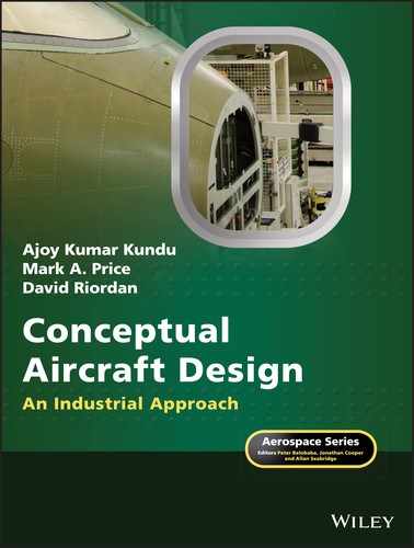
Post‐WWII research led to the rapid advancement of gas turbine development to a point when, from a core gas generator module, a family of engines could be made in a modular concept (Figure 12.1) that allows engine designers to offer engines as specified by the aircraft designers. Similar laws in thermodynamic design parameters permit power plants to be scaled (rubberised) to the requisite size around the core gas generator module to meet the demands of the mission requirements. The size and characteristics of engine is determined by matching with the aircraft mission. Now both the aircraft and the engine can be sized to the mission role, thereby improving operational economics. Modular engine design also favours low down times in maintenance.
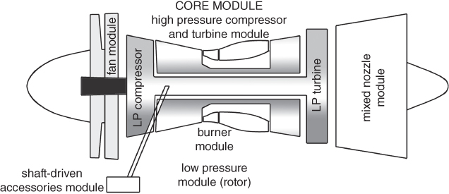
Figure 12.1 Modular concept of gas turbine design (the core module is also known as the gas generator module).
Potential energy locked in fuel is released through combustion in the form of heat energy. In gas turbine technology, the high energy of the combustion product can be used in two ways: (i) it is converted into increase in kinetic energy (KE) of the exhaust to produce the reactionary thrust (turbojet/turbofan) or (ii) it is further extracted through an additional turbine to drive a propeller (turboprop) to generate thrust.
Initially, the reactionary type engines came as simple straight‐through airflow turbojets (Figure 12.5). Subsequently, the turbojet development improved with addition of a fan (long compressor blades visible from outside) in front of the compressor and this type is called a turbofan. Commercial transport aircraft have a higher bypass ratio (BPR) (Section 12.3) requiring a large fan diameter, hence high drag and are they are pod mounted.
Gas turbine components' operating environment demands more complex aerodynamic considerations than aircraft. There are very high stress levels at considerably elevated temperature, yet it has to be made as light as possible, demanding stringent design considerations. Gas turbine parts manufacture is also a difficult task – very tough material has to be machined in a complex 3D shape to a very tight tolerance level (3D printing offers promise to alleviate some of these problems). All these considerations make gas turbine design a very complex technology, possibly second to none. Engine control also involves with very complex microprocessor based management.
Note that gas turbine engines have a wide range of applications from land based large prime movers for power generation and ship usages (civil and military) to weight critical airborne applications. The theories behind all the types have a common base – the hardware design differs, driven by the application requirements and technology level adopted – for example, land‐based gas turbines are not weight critical and do not have to stand alone; therefore, they are less constrained. Surface based gas turbines have to run economically for days/months generating a lot of power compared to standalone light aircraft engines running for hours in varying power, altitude, g‐load and airflow demands. Even the biggest aircraft gas turbine is small compared to the surface‐based ones.
Gas turbines design have advanced to incorporate sophisticated microprocessor‐based control system with automation, called FADEC (Full Authority Digital Engine Control) working in conjunction with fly‐by‐wire (FBW) control of aircraft. The uses of computer‐aided drawing (CAD)/computer‐aided manufacture (CAM)/computational fluid dynamics (CFD)/finite element method (FEM) are now the standard tools for engine design. Current developments involve having laminar flow in the intake duct, noise and emission reduction.
Liquid‐cooled aircraft piston engines over 3000 HP have been built. Except for a few types, they are no longer in production as they are too heavy for the power generated; in their place, gas turbines have taken over. Gas turbine engines have better thrust to weight ratio. Two of the successful piston engines were the WWII types – the Rolls Royce (RR) Merlin and Griffon. They produced 1000–1500HP and weighed around 1500 lb dry. Also, AVGAS (aviation gasoline‐petrol) is considerably more expensive than AVTUR (aviation turbine – kerosene). Today, the biggest aircraft piston engine in production is around 500 HP. Of late, diesel fuel piston engines (less than 250 HP) have entered the market for general aviation usage. In the home‐built market, MOGAS (automobile gasoline‐petrol) powered engines have appeared, approved by certification authorities. Battery powered small engines for very light aircraft are gaining ground (Chapter 24).
Chart 12.1 classifies all types of aircraft engines in current usage. Rocket propulsion is not included in this book.
Classification of aircraft engines.
Source: Reproduced with permission from Cambridge University Press.
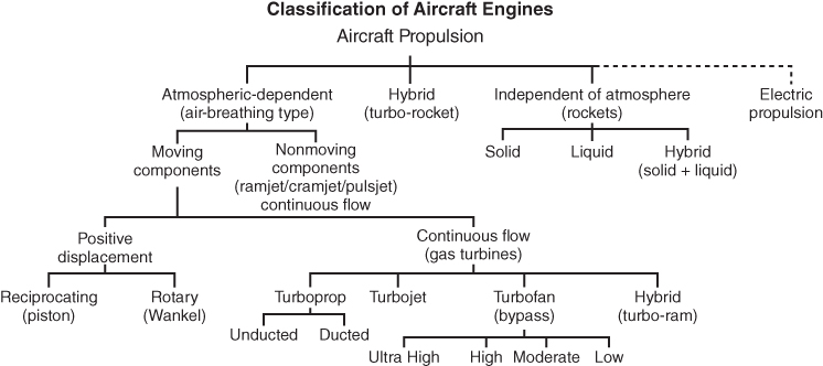
The application domain of the types dealt with in this book is shown in Figure 12.2 (excluding electric propulsion). High BPR turbofans are meant for high subsonic speeds. At supersonic speeds the bypass ratio comes down to less than three with the benefit of having smaller fan diameter that can be installed inside fuselage. Typically, turboprop powered aircraft speeds are around Mach 0.5 and below (higher speeds exceeding Mach 0.7 has been achieved). Piston engine powered aircraft are at the low speed end.
Figure 12.2 Application domains of various types of air‐breathing aircraft engines.
Turbofans (bypass turbojets) start to compete with turboprops for ranges over 1000 nm on account of time saved as a consequence of higher subsonic flight speed. Fuel cost is not the only consideration in a sector of operation. The combat aircraft power plant uses lower bypass turbofans with smaller fan diameters so that they can be installed within the aircraft fuselage, in earlier days they had straight‐through (no bypass) turbojets.
Figure 12.3a gives the thrust to weight ratio of various kind of engines. Figure 12.3b gives the specific fuel consumption (sfc) at sea level static takeoff thrust (TSLS) rating in International Standard Atmosphere (ISA) day of various classes of current engines. At cruise, sfc would be higher.

Figure 12.3 Engine performance. (a) Thrust to weight ratio and (b) specific fuel consumption (slightly modified from the diagrams in Aero Digest, Vol. 69, No. 1, July 1954).
Typical levels of specific thrust (F/![]() – lb (lb s)−1) and sfc – (lb (h lb)−1) of various types of gas turbines are shown Figure 12.4.
– lb (lb s)−1) and sfc – (lb (h lb)−1) of various types of gas turbines are shown Figure 12.4.

Figure 12.4 Typical performance levels of various gas turbine engines. (a) Specific thrust. (b) Specific fuel consumption.
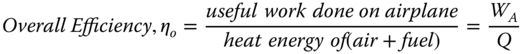
Table 12.1 gives various kinds of efficiencies of the different classes of aircraft engines. Table 12.2 gives progress made in the last half a century. It indicates considerable advances made in engine weight savings. Since the 1970s, the engine noise maximum level came into force as a requirement to comply with the certification authorisation. Pollution levels due to noise and emissions are steadily getting lower (Chapter 21).
Table 12.1 Efficiencies of engine types.
Source. Reproduced with permission from Cambridge University Press.
| Thermal efficiency | Propulsive efficiency | Overall efficiency | |
| Current types | 0.6–0.65 | 0.75–0.85 | 0.5–0.55 |
| Propfan | 0.52–0.55 | 0.8–0.85 | 0.54–0.55 |
| Propfan (ada ) | 0.52–0.55 | 0.7–0.76 | 0.46–0.5 |
| High BPR | 0.48–0.55 | 0.62–0.68 | 0.4–0.42 |
| Low BPR | 0.4–0.5 | 0.55–0.6 | 0.35–0.38 |
| Turbojet | 0.4–0.45 | 0.45–0.52 | 0.28–0.32 |
Advanced propfan.
Table 12.2 Progress in jet engines.
| Thrust/weight ratio | |
| 1950s (J69 class) | 2.8–3.2 |
| 1960s (JT8D, JT3D class) | 3.2–3.6 |
| 1970s (J79 class) | 4.5–7.0 |
| 1980s (TF34 class) | 6.0–6.5 |
| 1990s (F100, F404 class) | 7.0–8.0 |
| Current | 8.0–10.0 |
12.3 Definitions
The following are the definitions of various terminologies used in jet engine performance analysis.
Specific fuel consumption. This is the fuel flow rate required to produce one unit of thrust or shp.
Unit of sfc is in lb (h lb)−1 of thrust produced (in SI units – gm (s N)−1) – the lower the better. To be more precise, the reaction type engines use ‘tsfc’ and propeller‐driven ones use ‘psfc’, where, ‘t’ and ‘p’ stand for thrust and power, respectively. For turbofan engines,

Given next are the definitions of various kinds of efficiencies of jet engines. Subscript numbers indicate gas turbine component station numbers as shown in Figure 12.5 (in the figure, subscript 5 represents e).

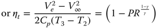

Figure 12.5 Sketch of a simple straight‐through turbojet (pod mounted turbojet from [2] – bare engine does not have intake and exhaust nozzle).
For a particular aircraft speed, V∞, the higher the exhaust velocity Ve, the better would be the ηt of the engine. Heat addition at the combustion chamber, q2–3 = Cp(T3 − T1) ≈ Cp(Tt3 − Tt1).

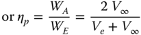
For subsonic aircraft, Ve » V∞. Clearly, for a given engine exhaust velocity, Ve, the higher the aircraft speed, the better the propulsion efficiency, ηp, will be. A jet aircraft flying below Mach 0.5 is not desirable – it is better to use propeller‐driven aircraft when flying at Mach 0.5 and below.
It can be shown [2–5] that for non‐afterburning (AB) engines, ideally the best overall efficiency, ηo, would be when the engine exhaust velocity, Ve, is twice the aircraft velocity, V∞. Bypassed turbofans offer such an opportunity at high subsonic aircraft speed.
12.3.1 Recovery Factor, RF
A bare engine on a ground test bed inhales free stream air directly and performs at its best. In contrast, an installed engine in an aircraft can only inhale the airflow diffused through the nacelle/intake duct incurring losses in the pressure head, expressed as recovery loss, defined next.
Intake Pressure Recovery Factor (RF),
where subscript ‘∞’ represents free stream condition and subscript ‘1’ represent fan face.
For pod mounted high subsonic jet aircraft at cruise Mach, RF is about 0.98.
For fuselage mounted side intake with engine at aft end, at subsonic Mach, RF is about 0.94–0.96.
For nose mounted pitot type long intake with engine at aft end, at subsonic Mach, RF is about 0.92–0.94.
At supersonic speed, shock loss has to be added (see Section 12.8.2).
12.4 Introduction – Air‐Breathing Aircraft Engine Types
This section starts with describing various types of gas turbines followed by introducing the piston engines. Aircraft propulsion depends on the extent of thrust produced by the engine. Chapter 13 presents the available thrust and power from various types of engines. Some statistics of various kinds of aircraft engines are given at the end of this chapter. Gas turbine sizes are progressing in making both larger and smaller engines than the current sizes, that is, expanding the application envelope.
12.4.1 Simple Straight‐Through Turbojets
The most elementary form of gas turbine is a simple straight‐through turbojet, as shown schematically in Figure 12.5. In this case, the intake airflow goes straight through the whole length of the engine and comes out at a higher velocity and temperature after going through the processes of compression, combustion and expansion. It burns like a stove under pressurised environment. The readers may note the waisting of the airflow passage as a result of compressor reducing the volume while the turbine expands. Typically, at long range cruise (LRC) condition, the free stream tube far upstream is narrower in diameter than at the compressor face. As a result, airflow ahead of the intake plane slows down as a pre‐compression phase.
Components associated with the thermodynamic processes within the engine are assigned with station numbers as given in Table 12.3.
Table 12.3 Gas turbine station number.
| Number | Station | Description |
| ∞ | Free stream | Far upstream (if pre‐compression is ignored than it is same as 0). |
| 0–1 | Intake | A short divergent duct as a diffuser to compress inhaled air mass. |
| 1–2 | Compressor | Active compression to increase pressure – temperature rises. |
| 2–3 | Burnera | Fuel is burned to release the heat energy. |
| 3–4 | Turbine | Extracts the power from heat energy to drive the compressor. |
| 4–5 | Nozzlea | Generally, convergent to increase flow velocity. |
| e | (station 5 is also known as ‘e’ representing the exit plane). |
Burner is also known as combustion chamber (CC) and the nozzle as exhaust duct.
Overall engine efficiency could be improved if the higher energy of the exhaust gas of a straight through turbojet is extracted through additional turbine that can drive an encased fan in front of a the compressor (when it is called turbofan engine) or a propeller (when it is called turboprop engine).
12.4.2 Turbofan – Bypass Engine (Two Flow – Primary and Secondary)
The energy extraction through the additional turbine lowers the rejected energy at the exhaust resulting in lower exhaust velocity, pressure and temperature. The additional turbine drives a fan in front of q compressor. A large amount of air mass flow through the fan provides thrust. The intake air mass flow is split into two streams (Figure 12.6), the core airflow passes through the combustion chamber of the engine as primary flow and is made to burn while the secondary flow through the fan is bypassed (hence also called bypass engine) around the engine and remains as cold flow. It is for this reason that primary flow is also known as hot flow and the secondary bypassed flow as cold flow. Figure 12.6b gives a schematic diagram of a turbofan engine (top Figure 12.6a is that of bare PW 2037 turbofan). Lower exhaust velocity reduces engine noise. At the design point (LRC), lower exhaust pressure permits the nozzle exit area to be sized to make exit pressure equal to ambient pressure (perfectly expanded nozzle), unlike simple turbojets that can have higher exit pressure.
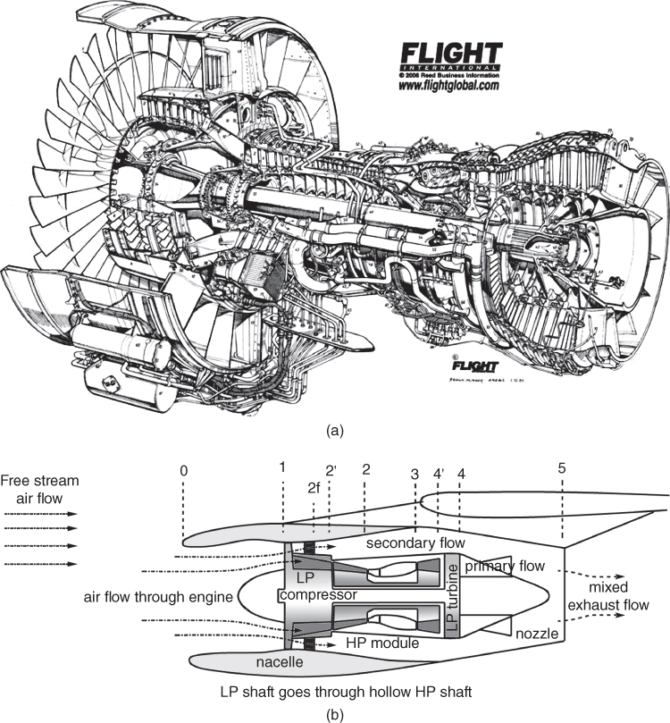
Figure 12.6 Turbofan engine. (a) Pratt and Whitney 2037 Turbofan (Credit: Flightglobal). (b) Schematic diagram of a pod mounted long duct two‐shaft turbofan engine.
Source: Reproduced with permission from Flightglobal.
The readers may note that the component station numbering system follows the same pattern as for the simple straight‐through turbojet. The combustion chamber in the middle maintains the same numbers of 2–3. The only difference is the fan exit is with subscript of ‘f’. Intermediate stages of compressor and turbine are primed (′).
Typically, the BPR – (Eq. 12.2) for commercial jet aircraft turbofans (high subsonic flight speed of less than 0.98 Mach) is around 4–6 with large fan face diameter and are invariably pod mounted. Of late, turbofans for the new B787 have exceeded a BPR of 8. Airbus 350 and Bombardier C‐series turbofans have a BPR = 12. For military application (supersonic flight speed up to Mach 2.5), the BPR is around 1–3. Lower BPR keeps the fan diameter smaller and hence lowers frontal drag so it can be integrated within fuselage.
Multi‐spool (shaft) drive shafts offer better efficiency and response characteristics, mostly with two concentric shafts. The shaft driving the low‐pressure (LP) section runs inside the hollow shaft high‐pressure (HP) section – see the diagram in Figure 12.6. Three shaft turbofans have been designed, but most of the current designs have a twin spool. The recent advent of a geared turbofan offers better fuel efficiency.
Lower fan diameter compared to the propeller permits higher rotational speed and offers scope for having a thinner aerofoil section to extract better aerodynamic benefits. The higher the BPR, the better the fuel economy. Higher BPR demands a larger fan diameter when reduction gears may be required to keep the rpm at a desired level. Ultra‐high bypass ratio (UHBPR) turbofans approach the class of ducted fan or ducted propeller or propfan engines. Such engines have been built but their cost versus performance is yet to break into the market arena.
12.4.3 Three Flow Bypass Engine
While the two streams (primary hot core flow and the secondary cold high bypass flow) offer good fuel economy for the high subsonic transport category aircraft operation, they are not is suitable for supersonic military application due to having a large fan face diameter generating high drag. High BPR specific thrust is considerably lower than low bypass ratio of military jet engines. Of current interest for supersonic combat class aircraft engine is pursuing the concept of the adaptive three‐stream bypass jet engine. This improves the fuel economy while keeping the front fan face diameter relatively small.
The adaptive three‐stream jet engine has the third outer flow as a second layer of bypass over the conventional two stream bypass turbofan. The adaptive three‐stream jet engine is a variable cycle engine, because the third airflow stream has a movable internal inlet door that can adjust the second bypass flow during the flight to suit the mission demand. The outer cold third air stream also serves for thermal management of the hot combustion product primary core flow and abates the noise level as well. This arrangement shows improved fuel economy while retaining high specific thrust suiting supersonic military combat aircraft operation. This type of engine is currently in the developmental stage with a technology demonstrator running under test.
12.4.4 Afterburner Engines
The AB is another method of thrust augmentation exclusively meant for supersonic combat category aircraft (the Concorde is the only civil aircraft to use an AB). Figure 12.7 gives a cutaway diagram of a modern AB meant for combat aircraft.

Figure 12.7 Afterburning engine – Volve‐Flygmotor RM8 (Credit: Flightglobal).
Source: Reproduced with permission from Flightglobal.
The simple straight‐through turbojets or low bypass ratio turbofans have a relatively small frontal area to give low drag and have excess air in the exhaust flow. If additional fuel can be burned in the exhaust nozzle beyond the turbine exit plane, then additional thrust can be generated to propel the aircraft at a considerably higher speed and acceleration, thereby also giving the chance to improve propulsive efficiency. However, the reason for using AB arises from the mission demand, for example, at takeoff with high payload, acceleration to engage/disengage during combat/evasion manoeuvres and so on. Mission demand overrides the fact that there is a very high level of energy rejection in the high exhaust velocity. The fuel economy with AB degrades – it takes 80–120% higher fuel burn to gain 30–50% increase in thrust. Nowadays, most supersonic aircraft engines have some BPR when afterburning can be done within in the cooler mixed flow past the turbine section of the primary flow.
12.4.5 Turboprop Engines
Lower speed aircraft could use propellers for thrust generation. Therefore, instead of driving a smaller encased fan (turbofan), a large propeller (known as a turboprop) can be driven by gas turbine to improve efficiency as the exhaust energy can be further extracted to very low exhaust velocity (nearly zero nozzle thrust) (Figure 12.8). There could be some residual jet thrust left at the nozzle exit plane when it needs to be added to the propeller thrust. The nozzle thrust is converted into HP and together with the shaft horse power (SHP) generated; it becomes Equivalent Shaft Horse Power (ESHP).
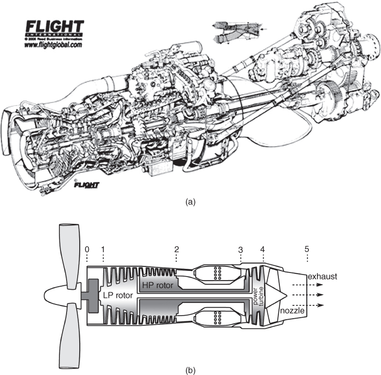
Figure 12.8 Aircraft turboprop engine. (a) General Electric CT7 (Credit: Flightglobal). (b) Schematic drawing of a turboprop engine.
Source: Reproduced with permission from Flightglobal.
However, a large propeller diameter would limit rotational speed on account of both aerodynamic (transonic blade tips) and structural considerations (centrifugal force). The relative velocity with respect to the propeller blade is the resultant velocity (Figure 12.24) of aircraft speed and the propeller rpm can reach a transonic level when propeller efficiency suffers on account of compressibility effects and possibly trailing edge separation as a result of local shock and boundary layer interaction. Heavy reduction gears are required to bring down propeller rpm to a desirable level. Propeller efficiency drops when aircraft operate at flight speeds above Mach 0.7. For shorter range flights, the turboprop's slower speed does not become time critical to the user and yet it offers better fuel economy. Military transport aircraft are not as time critical as commercial transport and may use a turboprop (e.g. A400). Figure 12.8 gives a schematic diagram of typical turboprop engines. Modern turboprops have up to eight blades (see Section 12.10) allowing reduction of diameter size and operation at a relatively higher rpm. Advanced propeller designs permit aircraft to fly above Mach 0.7.
12.4.6 Piston Engines
Most of the aircraft piston engines are reciprocating types (positive displacement – intermittent combustion), the smaller ones are air‐cooled two‐stroke cycle – the bigger ones (typically over 200 HP) are liquid‐cooled four‐stroke cycle. There are a few rotary type positive displacement engines (Wankel) – in principle, they very attractive but they have some sealing problems. Cost wise, the rotary type positive displacement engines are not popular yet on account of these sealing problems. Cost goes down with an increase in the number of production. Figure 12.9 shows aircraft piston engine with its installation components.
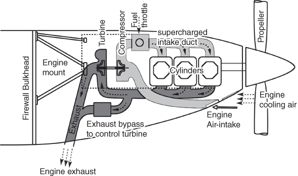
Figure 12.9 Aircraft piston engine and the supercharged scheme.
To improve high altitude performance (having low air density) supercharging is used. Figure 12.9 shows vane supercharging type for pre‐compression. Also aviation fuel (AVGAS – petrol) differs slightly from automobile petrol (MOGAS). Of late, some engines for the home‐built category are to use MOGAS. Recently, small diesel engines have been introduced on the market.
Piston engines are the oldest type to power aircraft. Over the life‐cycle of an aircraft, gas turbines prove more cost effective for engine sizes over 500 HP. Currently, general aviation aircraft are the main users of piston engines. Recreational small aircraft are invariably powered by piston engines.
12.5 Simplified Representation of a Gas Turbine (Brayton/Joule) Cycle
Figure 12.10a depicts a standard schematic diagram representing a simple straight through turbojet engine as shown in Figure 12.5, with the appropriate station numbers. The thermodynamic cycle associated with gas turbines is known as Joule cycle (also known as Brayton cycle). Figure 12.10b gives the corresponding temperature‐entropy diagram of an ideal Joule cycle in which isentropic compression and expansion takes place.

Figure 12.10 Simple straight‐through jet. (a) Generic schematic diagram. (b) Ideal Joule cycle.
Real engine processes are not isentropic and there are losses involved associated with increased entropy. Comparison of real and ideal cycle is shown in Figure 12.11.
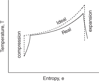
Figure 12.11 Real and Ideal Joule (Brayton) cycle comparison of a straight‐through jet.
12.6 Formulation/Theory – Isentropic Case (Trend Analysis)
The basic thermodynamic relationships and the related gas turbine equations pertinent to this book are given in Appendix C. These are valid for all types of processes. For more details, see [2–5, 7, 8].
12.6.1 Simple Straight‐Through Turbojet Engine – Formulation
Consider a control volume (CV – dashed line – note the waist like shape the bare simple turbojet) representing a straight through axi‐symmetric turbojet engine as shown in Figure 12.12. The CV and the component station numbers are as per the sketch and convention shown in Figure 12.6. Gas turbine intake starts with a subscript 0 or ∞ and ends at the nozzle exit plane with subscript 5 or e. Free stream air mass flow rate (MFR), ![]() , is inhaled into the CV at the front face perpendicular to the flow and fuel MFR
, is inhaled into the CV at the front face perpendicular to the flow and fuel MFR ![]() (taken from the onboard fuel tank) is added at the combustion chamber and the product flow rate
(taken from the onboard fuel tank) is added at the combustion chamber and the product flow rate ![]() is exhausted out of the nozzle plane perpendicular to flow. It is assumed that inlet face static pressure is p∞, which is fairly accurate. Pre‐compression exists but for ideal consideration it has no loss.
is exhausted out of the nozzle plane perpendicular to flow. It is assumed that inlet face static pressure is p∞, which is fairly accurate. Pre‐compression exists but for ideal consideration it has no loss.

Figure 12.12 Control volume (CV) representation of straight‐through turbojet.
No flow crosses the other two lateral boundaries of the CV as it is aligned with the walls of the engine. Force experienced by this CV is the thrust produced by the engine. Consider a cruise condition with aircraft velocity of V∞. At cruise, the demand for air inhalation is considerably lower than at takeoff. Intake area is sized in between the two demands. At cruise the intake stream tube cross‐sectional area is smaller than the intake face area – it is closer to that of exit plane area, Ae (gas exiting at very high velocity). Since this is under ideal conditions, there is no pre‐compression loss, station 0 may be considered as having free stream properties with subscript ∞.
From Newton's second Law,
Applied force, F = rate of change of momentum + net pressure force.
Note that the momentum rate is given by the MFR.
Therefore,
Net pressure force between the intake and exit planes = (peAe − p∞A∞). The axi‐symmetric side pressure at the CV walls cancels out. Typically, at cruise, sufficiently upstream Ae ≈ A∞.
Therefore,
Then
And ![]() V∞ = Ram drag (with a −ve sign, it has to be drag). It is the loss of momentum seen as drag on account of slowing down of the income air as ram effect.
V∞ = Ram drag (with a −ve sign, it has to be drag). It is the loss of momentum seen as drag on account of slowing down of the income air as ram effect.
This gives,
Ae (pe − p∞) = pressure thrust. In general, subsonic commercial transport turbofans have convergent nozzle, its exit area is sized in a way that in cruise, pe ≈ p∞ (known as a perfectly expanded nozzle). It is different for military engines especially with afterburning, when pe > p∞, thus requiring a convergent‐divergent nozzle.
For a perfectly expanded nozzle (pe − p∞),
Further simplification is possible by ignoring the effect of fuel flow, ![]() , since
, since ![]() »
» ![]() .
.
Then the thrust for perfectly expanded nozzle is,
At sea level static takeoff thrust (TSLS) ratings V∞ = 0,
which makes,
The expression indicates that the thrust increase can be achieved by increasing intake air MFR and/or increasing exit velocity.
Equation 12.4 gives propulsive efficiency,
 12.11
12.11
Clearly, a jet propelled aircraft with low flight speed will have poor propulsive efficiency, ηp. Jet propulsion is favoured for aircraft flight speed above Mach 0.6.
The next question is where does the thrust act? Figure 12.13 [1] shows a typical gas turbine where the thrust is acting. It is all over the engine and the aircraft realises the net thrust transmitted through the engine‐mount bolts.

Figure 12.13 Where does the thrust act? [1].
12.6.2 Bypass Turbofan Engines – Formulation
Typically, in this book a long duct nacelle is preferred to obtain better thrust and fuel economy offsetting the weight gain as compared to short duct nacelles (see Figure 12.17). Note that pressure rise across fan (secondary cold flow) is substantially lower than pressure rise of the primary airflow. Also note that the secondary airflow does not have heat addition as in the primary flow. The cooler and lower exit pressure of the fan exit, when mixed with the primary hot flow within the long duct, brings the final pressure lower than the critical pressure (Ve just reaches sonic speed) favouring a perfectly expanded exit nozzle (pe = p∞). Through mixing, there is reduction in jet velocity, which offers a vital benefit of noise reduction to meet the airworthiness requirements. A long duct nacelle exit plane can be sized to expand perfectly.
Primary flow has a subscript designation of p and secondary flow has a subscript designation of s. Therefore, Fp and Vep stand for primary flow thrust and exit velocity, respectively, and Fs and Ves stand for bypass‐flow thrust and its exit velocity, respectively. Thrust (F) equations of perfectly expanded turbofans are separately computed for primary and secondary flows, and then added to obtain the net thrust, F, of the engine (perfectly expanded nozzle, i.e. pe = p∞).
Specific thrust in terms of primary flow becomes (f = fuel to air ratio)
If fuel flow is ignored, then
![]()
or
At a given design point, that is, BPR, flight speed V∞, fuel consumption, and ![]() are held constant. Then the best specific thrust and KE can be found by varying the fan exit velocity for a given Vep. This is when setting their differentiation with respect to Ves equal to zero. (This may be taken as trend analysis for ideal turbofan engines. The real engine analysis is more complex.)
are held constant. Then the best specific thrust and KE can be found by varying the fan exit velocity for a given Vep. This is when setting their differentiation with respect to Ves equal to zero. (This may be taken as trend analysis for ideal turbofan engines. The real engine analysis is more complex.)
Then by differentiating Eq. 12.13,
And Eq. 12.14 becomes
Combine Eqs. 12.15 and 12.16,
And since BPR ≠ 0, then the optimum has to be when
that is, the best specific thrust is when the primary (hot core flow) exit flow velocity equals the secondary (cold fan flow) exit flow velocity.
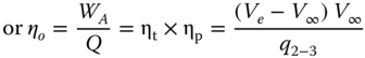
Equation 12.4 gave turbojet propulsive efficiency, ηp = ![]() for a simple turbojet engine, but in the case of a turbofan there are two exit plane velocities: one each for hot core primary flow (Vep) and cold fan secondary flow (Ves). Therefore, an equivalent mixed turbofan exit velocity (Veq) could substitute for Ve in Eq. 12.4. Fuel flow rates are small and can be ignored. The equivalent turbofan exit velocity (Veq) is obtained by equating the total thrust (perfectly expanded nozzle) as if it is a turbojet engine with total mass flow (
for a simple turbojet engine, but in the case of a turbofan there are two exit plane velocities: one each for hot core primary flow (Vep) and cold fan secondary flow (Ves). Therefore, an equivalent mixed turbofan exit velocity (Veq) could substitute for Ve in Eq. 12.4. Fuel flow rates are small and can be ignored. The equivalent turbofan exit velocity (Veq) is obtained by equating the total thrust (perfectly expanded nozzle) as if it is a turbojet engine with total mass flow (![]() +
+ ![]() ):
):
Thus
Then turbofan propulsive efficiency,
Large engines could benefit from weight savings by installing short duct turbofans.
12.6.3 Afterburner Engines – Formulation
Figure 12.14 gives a schematic diagram with the station numbers for the afterburning jet engine. To keep numbers consistent with the turbojet numbering system, there is no difference between stations 4 and 5 representing turbine exit condition. Station 5 is the start and station 6 is the end of afterburning. Station 7 is the final exit plane. Figure 12.14 also shows the real cycle of afterburning in a T‐s diagram.

Figure 12.14 Afterburning turbojet and its T‐s diagram (real cycle).
Afterburning is deployed only in military vehicles (except in the supersonic Concorde aircraft) as a temporary thrust augmentation device to meet mission demand at takeoff and/or for fast acceleration/manoeuvre to engage/disengage in combat. Afterburning is applied at full throttle by flicking a fuel switch. The pilot can feel its deployment with sudden increase in ‘g’ level in the flight direction. The ground observer would notice a sudden increase in noise level, which can exceed the physical threshold. Afterburning glow is visible at the exit nozzle, in darkness it is depicted as a spectacular plume with supersonic expansion diamonds. In the absence of any downstream rotating machines, the afterburning temperature limit can be raised to around 2000–2200 K at the expense of a large increase in fuel flow (a richer fuel/air ratio than in the core combustion).
The afterburning exit nozzle would invariably run choked (at sonic speed) and would require a convergent‐divergent nozzle to make supersonic expansion to increase gain in momentum for thrust augmentation. Typically, to gain a 50% thrust increase, fuel consumption increases by about 80–120%. That is why it is used for short periods, not necessarily in one burst. Interestingly enough, afterburning in bypass engines is an attractive proposition because afterburning inlet temperature is lower. In fact, all modern combat category engines use a low BPR of 1–3 resulting in a smaller frontal area suited to in‐fuselage installation.
Losses in afterburning exit nozzles are high – the flame holders and act as obstructions. It is desirable to diffuse flow speed at the afterburner to around 0.2–0.3 Mach – this results in a small bulge in the jet pipe diameter around that area. The combat aircraft fuselage has to house this.
12.6.4 Turboprop Engines – Formulation
Section 12.4.4 described turboprops. It has considerable similarity with turbojets/turbofans except that the high energy of exhaust jet is utilised to drive a propeller by incorporating additional low‐pressure turbine stages as shown in Figure 12.8. Thrust developed by the propellers is the propulsive force for the aircraft. There could be a small amount of residual thrust left at the nozzle exit plane that should be added to the propeller thrust. The relation between thrust power (TP) and gas turbine shaft power (SHP) is related to the propeller efficiency, ηprop as:
ESHP is a convenient way to define the combination of shaft and jet power as follows:
Evidently, aircraft at the static condition will have ESHP = SHP, as the small thrust at the exit nozzle is not utilised. As speed increases, ESHP > SHP as long as there is some thrust at the nozzle. Power specific fuel consumption (psfc) and specific power (weight‐to‐power ratio) are expressed in terms of ESHP.
12.6.4.1 Summary
The formulae give good reasoning on the gas turbine domain of application as shown in Figure 12.2. Turboprops would offer the best economy for design flight speeds at Mach 0.5 and below, suited well to shorter ranges of operation. At higher speeds up to Mach 0.98, turbofans with a high BPR offer better efficiencies (see comments followed after Eq. 12.5). At supersonic speeds, the BPR is reduced and in most cases an afterburner used. Small aircraft with piston engines up to a size (≈≤ 500 HP) that gas turbine can compete with.
12.7 Engine Integration to Aircraft – Installation Effects
Engine manufacturers supply bare engines to the aircraft manufacturers who install them on to aircraft to integrate. The same type of engines could be used by different aircraft manufacturers who each have their own integration requirements. Engine installation on to aircraft is a specialised technology that aircraft designers must know. Engine integration is carried out by the aircraft manufacturers in consultation with the engine manufacturer. Positioning of the nacelle/intake with respect to aircraft/wing is dealt with in detail in Chapter 8.
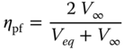
A bare engine at the test stand performs differently to an installed engine on an aircraft. Installation effects of engines are those arising from having a nacelle, that is, the losses of intake and exhaust plus off‐takes of power (to drive motor/generators etc.) and air bleeds (anti‐icing, environmental control etc.) Total loss of thrust at takeoff can be as high as 8–10% of that generated by a bare engine at test bed. At cruise, it can be brought down to less than 5%. Figure 12.15 shows typical off‐takes required on account of various installation effects. Aircraft performance engineers use installed engine performance.
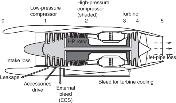
Figure 12.15 Installation effects.
Aircraft performance engineers must be given the following data to generate installed engine performance:
- Intake and jet pipe losses.
- Compressor air‐bleed for the Environmental Control Systems (ECSs), for example, cabin air‐conditioning and pressurisation, de‐icing/anti‐icing and any other purpose.
- Power off‐takes from engine shaft to drive electric generator, accessories and so on.
The nacelle is the housing for the engine and interfaces with the aircraft; typically, it would be a pod mount for civil aircraft design. Aircraft with more than one engine would have the pod mounted on the wing and/or on fuselage. It was mentioned earlier that wing mounted nacelles are the best to relieve wing bending under in‐flight load. Propeller‐driven engine nacelles also have a similar consideration of podded nacelles, modified by the presence of a propeller (Section 12.7.2). Aircraft with one engine are aligned in the plane of aircraft symmetry (engines with propellers can have a small lateral inclination of a degree or two about the aircraft centreline to counter the slipstream and gyroscopic effects from a rotating propeller). Position of the nacelles with respect to the aircraft and their shaping to reduce drag are the important considerations. Military aircraft have engines buried into the fuselage so they do not have nacelles unless designers choose to have pods (some older designs). Military aircraft designers are only to consider intake design as discussed in Section 12.7.3.
12.7.1 Subsonic Civil Aircraft Nacelle and Engine Installation
The nacelle is a multi‐functional system comprising of (i) inlet, (ii) exhaust nozzle, (iii) TR, if required and (iv) noise suppression system. The design aim of the nacelle is to minimise associated drag, noise and provide airflow smoothly to the engine at all flight conditions.
As of today, except for Concorde, all civil aircraft are subsonic with a maximum speed less than Mach 0.98. All subsonic aircraft use some form of pod mounted nacelle, in a way this has become generic in design. Figure 12.16 shows a turbofan installed in a civil aircraft nacelle pod. The under‐wing nacelle is the current best practice but for smaller aircraft, ground clearance issues force a nacelle to be fuselage mounted. An over‐wing nacelle like that of VFW614 is a possibility yet to be explored properly (Honda jet aircraft have reintroduced it).
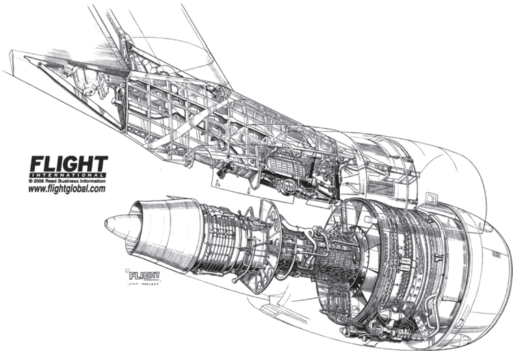
Figure 12.16 Installed turbofan on an aircraft (Credit: Flightglobal).
Source: Reproduced with permission from Flightglobal.
There are two types of podded nacelles. Figure 12.17a shows a long duct nacelle where both the primary and secondary flows mix within it. The mixing increases the thrust and reduces the noise level compared to the short duct nacelles, possibly compensating the weight gain through fuel and cost saving. Figure 12.17b shows short duct nacelle in which the bypassed cold flow does not mix with the hot core flow. The advantage is that there is considerable weight saving by cutting down the length of the outside casing of the nacelle by not extending up to the end. Short duct nacelle length can vary.
Figure 12.17 Podded nacelle types (courtesy of Bombardier‐Aerospace Shorts).
The aircraft performance engineers are to substantiate to the certification authorities that the thrust available from the engine after deducting the losses is sufficient to cater for the full flight envelope as specified. In hot and high altitude conditions, it can become critical at aircraft takeoff if (i) the runway is not sufficiently long and/or at high altitude, (ii) if there is an obstruction to clear or (iii) ambient temperature is high. In that case, the aircraft may takeoff with lighter weight. Airworthiness requirements require that the aircraft has to maintain a minimum gradient (Chapter 15) at takeoff with the critical one engine inoperative. Customer requirements could demand more than the minimum requirements.
12.7.2 Turboprop Integration to Aircraft
The turboprop nacelle is also a multi‐functional system comprising of (i) inlet, (ii) exhaust nozzle and (iii) noise suppression system. Thrust reversing can be achieved by changing the propeller pitch angle sufficiently. There are primarily two types of turboprop nacelles as shown in Figure 12.18. The scoop intake could be above or below (as a chin) the propeller spinner. Interestingly, quite a few turboprop nacelles have an integrated undercarriage mount with storage space in the same nacelle housing as can be seen in Figure 12.18a. The other kind is with annular intake as shown in Figure 12.18b. Installation losses are of the same order as discussed in the turbofan installation.

Figure 12.18 Typical wing mounted turboprop installation [9]. (a) Scoop intake. (b) Annular Intake.
Source: Reproduced with permission from Flightglobal.
Turboprop nacelle position is dictated by the propeller diameter. The key geometric parameters for turboprop installation are shown in Figure 12.19.
Figure 12.19 Typical turboprop installation parameters. (a) Wing mounted turboprop (note overhang). (b) Fuselage mounted turboprop.
Figure 12.19a shows wing mounted turboprop installation. Overhang should be as far forward the design can take, like that of turbofan overhang to reduce interference drag. For high wing aircraft, the turboprop nacelle is generally under the wing, like the Bombardier Q400 aircraft. For low wing aircraft, nacelles are generally over the wing to get propeller ground clearance. Both types can house the undercarriage. The propeller slipstream assists lift and has a strong effect on static stability, flap deployment aggravates the stability changes. Depending on the extent of wing incidence with respect to the fuselage, there is some angle between wing chord line and the thrust line – typically from 2 to 5°.
A fuselage mounted propeller‐driven system arrangement is shown in Figure 12.19b. Note the angle between the thrust line and the wing chord line as it is with wing mounted propeller nacelle. Sometimes, propeller axis is given about a degree down inclination with respect to fuselage axis. This assists longitudinal stability. To counter the propeller slipstream effect, an inclination of a degree or two in the yaw direction can be given. Otherwise, the V‐tail can be given such inclination to counter the effect.
Piston engine nacelles on the wing follow the same logic. The older designs had more closely coupled installations.
12.7.3 Combat Aircraft Engine Installation
A combat aircraft has engines integral with the fuselage, mostly buried inside but in some cases, with two engines, they can bulge out to the sides. Therefore, pods do not feature unless they are required for having more than two engines on a large aircraft. Figure 12.20 shows a turbofan installed on to a supersonic combat aircraft.
Figure 12.20 Installed engine in a combat aircraft [9].
The external contour of the engine housing is integral to fuselage mouldlines. Early designs had the intake at the front of the aircraft; a pitot type for a subsonic fighter (Sabrejet F86 etc.) and with a movable centre body for a supersonic fighter (MIG 21). The long intake duct snaking inside the fuselage below the pilot seat incurs high losses. Side intakes overtook nose intake designs. A possible choice for side intakes is given in Section 5.12 – primarily, they are side or chin mounted. A plate is kept above the fuselage boundary layer on which the intake is placed. A centre body is required for aircraft speed capability above Mach 1.8, otherwise it can be a pitot intake.
Aircraft performance engineers must be given the following data to generate the installed engine performance.
- Intake losses plus losses arising from supersonic shock waves and the duct length.
- Exit nozzle losses. Military aircraft nozzle design is complex.
- Additional losses at the intake and nozzle on account of suppression of exhaust temperature for stealth.
- Compressor air‐bleed for the ECSs, for example, cabin air‐conditioning and pressurisation, de‐/anti‐icing and any other purpose.
- Power off‐takes from the engine shaft to drive the electric generator, accessories, for example, pumps and so on.
Military aircraft have excess thrust (with or without afterburner) to cater for hot and high‐altitude conditions and operating from short airfields, and they are capable of climbing at steeper angles than civil aircraft. When thrust/weight ratio is more than 1, then the aircraft is able to climb up vertically.
12.8 Intake/Nozzle Design
Since the withdrawal of supersonic Concorde, there is currently no supersonic civil aircraft in operation. This section separates subsonic and supersonic intakes as civil and military operational applications, respectively.
12.8.1 Civil Aircraft Subsonic Intake Design
Engine mass flow demand varies a lot as shown in Figure 12.21. To size intake area, the reference cross‐section of incoming air mass stream tube is taken at the maximum cruise condition as shown in Figure 12.21a, when it has cross‐sectional area almost equal to that of highlight area (i.e. A∞ = A1). The ratio of MFR in relation with the reference condition (air mass flow at maximum cruise) is a measure of spread the intake would encounter. At the maximum cruise condition, MFR = 1 as a result of A∞ = A1 (critical operation). At normal cruise conditions the intake air mass demand is lower (MFR < 1 (sub‐critical operation), shown in Figure 12.21b). At the maximum at takeoff rating (MFR > 1), intake air mass flow demand is high and the streamline patterns is shown in Figure 12.21c. Variation in intake mass flow demand is quite high.
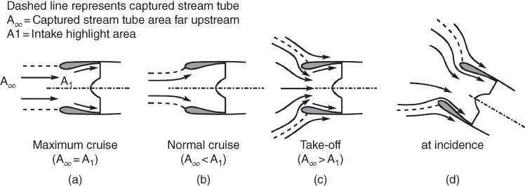
Figure 12.21 Subsonic intake airflow demand (valid both for civil and military intakes). (a) MFR ratio = 1. (b) MFR ratio < 1. (c) MFR ratio > 1. (d) MFR ratio > 1 (at climb).
If the takeoff airflow demand is high enough then a blow‐in door can be provided, which closes automatically when the demand drops off. Figure 12.21d shows a typical flow pattern at incidence at high demand, when an automatic blow‐in door may be necessary. At idle, the engine is kept running with very little trust generation (MFR « 1). At inoperative conditions, the rotor is kept windmilling to minimise drag. If the rotor seizes due to mechanical failure then there will be considerable drag rise.
Currently, the engine (fan) face Mach number should not exceed Mach 0.5 to avoid degradation due to compressibility effects. At a fan face Mach number above 0.5, the relative velocity at the fan tip region approaches near sonic speed on account of high blade rotational speed.
The purpose of the intake is to serve engine airflow demand as smoothly as it is possible – there should be no flow distortion at the compressor face on account of any separation and/or flow asymmetry. Nacelle intake lip cross‐section is designed with the similar logic behind designing the aerofoil leading edge cross‐section – to ensure flow does not separate within the flight envelope. More detail on subsonic pod mounted intake design is given in [8–10].
12.8.2 Military Aircraft Supersonic Intake Design
Chart described various types of supersonic inlet configurations shown in Section 5.16.1. The two main types are featured at the (i) fuselage nose with a centre body and (ii) fuselage, side mounted. In this section, their aerodynamic considerations are given. Military aircraft have supersonic capabilities and therefore have to manage shock losses (RF, Eq. 12.6 and Figure 12.22) associated with its intake. This can be done by designing supersonic intake oblique shock to develop in stages with a series of deflection angles (typically 5–10°, depending on the number of stages). Normally, three oblique shocks suffice (Figure 12.22) [6, 10]. An increase in number of deflection angles offers diminishing returns to improve RF. The best design is an Oswatitsch curved contour design, which generates infinite weak Mach waves with minimum loss, ideally in an isentropic process; that is, no loss. Oswatitsch intakes are used in hypersonic air‐breathing engines.
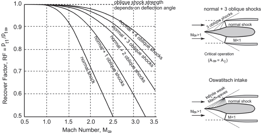
Figure 12.22 Shock Recovery Factor, RF.
12.8.2.1 Intake at Fuselage Nose with a Centre Body
Ideally, at design point Mdes, (at supersonic cruise), the bow shock wave just attaches to the intake lip, which is sharp compared to a subsonic intake lip. Figure 12.23 gives four kinds of flow regime associated with supersonic intake with a fixed centre body. Four types of operating situation arise as follows:
- At the design flight speed, seen as critical operation, when it is desirable that the oblique shock wave just touches the lip followed by other shocks culminating with a normal shock at the throat beyond which airflow becomes subsonic (Figure 12.23a). The captured free stream tube is same as the highlight area. Intake area is sized to inhale air mass at critical operation.
- If the back pressure is lower than the critical operation (on account of throttle action) then more air mass is inhaled and the throat area remains supersonic, pushing back a stronger normal shock. This is known as supercritical operation (Figure 12.23b). The captured free stream tube is still the same as the highlight area and oblique shock position depends on the aircraft speed.
- When the back pressure is high, especially when the aircraft is below critical speed, then less air is inhaled, the aircraft is still at supersonic speed, the oblique shock is wider and is followed by a normal shock that pops outside ahead of the nacelle lip and is known as the sub‐critical operation (Figure 12.23c). The captured free stream tube is smaller than the highlight area. It is not as efficient as the critical operation but loss is less than supercritical operation.
- The last one could happen with a particular combination of aircraft speed (below critical) and air mass inhalation when the normal shock outside keeps oscillating, which starves the engine and it runs erratically, possibly leading to flameout. This is known ‘buzz’ (Figure 12.23d).

Figure 12.23 Types of ideal supersonic intake demand conditions [6]. (The Schlieren image is that of the buzz phenomenon, the left image has shock inside, then progressing to emerge to its extreme position at the right image and cycles in about 15 Hz [6].)
For aircraft operating above Mach 2, a movable centre body keeps the oblique wave at the lip as the shock angle changes with speed change. The simplest centre body is a cone (or half cone for side mounted nacelles). The cone could be stepped to make multiple oblique shocks at reduced intensity; that is, lowering shock loss. A movable centre body (Figure 5.34, MIG21 showing extended and retracted centre body positions) can keep oblique shock at the intake lip and can manage ‘buzz’ better. Aircraft must avoid buzz occurring and modern designs have a FBW/FADEC to keep clear of it.
12.8.2.2 Intake at the Fuselage Side
Current intake position is at fuselage side or at underbelly, reducing the long intake duct of nose intake by about 25–35%, reducing duct loss and duct weight. For fuselage mounted single engine, a small bend of intake duct is required to have the bifurcated duct to meet before it reaches engine face. For twin engine aircraft, relatively straighter separate ducts offer better design with less duct loss, thus offering better RF. A chin mounted intake escapes duct bifurcation.
Figure 12.24 shows a typical side mounted supersonic intake similar to what an F14 Tomcat fighter aircraft has. It has a rectangular intake seen as a 2D intake, but not exactly. The Concorde underwing supersonic intake has similar design considerations.
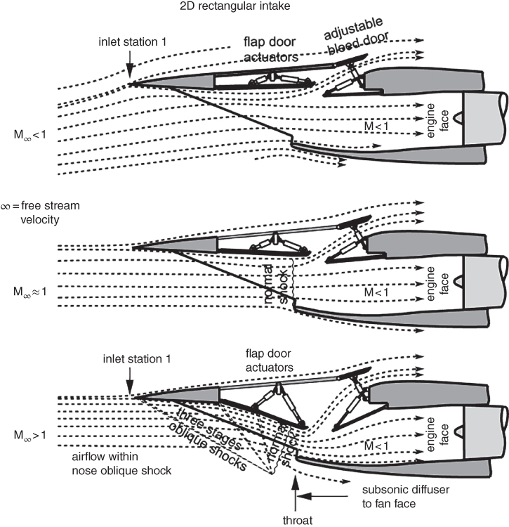
Figure 12.24 Types of ideal supersonic intake demand mechanism [6].
The supersonic nacelle, as shown in Figure 12.24, is a complex modern design. It dispenses with the older practices of having a centre body by movable doors operated by separately managed actuators. For mass flow demand at low speed operation, especially, at full throttle takeoff rating, the throat opening is kept at maximum. Flap doors are adjusted to reduce throat area with speed increase. At maximum speeds over Mach 2.0, the two stage doors have stepped deflection to develop a total of three weaker oblique shocks, followed by a normal shock, making airflow diffuse to around Mach 0.5 at the engine face. At the top, there is a bleed door to serve both as boundary layer bleed as well as a dumping excess intake air mass flow. Normally, these are integrated with FBW/FADEC and activate automatically.
Modern combat aircraft with advance missiles have beyond visual range (BVR) capabilities. In an air‐superiority role, rapid manoeuvre at high speed is the combat specification for which a typical maximum speed is of the order of Mach 1.8 (≈F16 variant) when the requirement for a movable centre body/flap doors is not stringent. For side intakes, boundary layer bleed plates serve as the centre body to position oblique shock at the lip (critical design point operation). A Diverterless Supersonic Inlet (DSI – Figure 5.33) eliminates the need for a splitter plate, while compressing the air to slow it down from supersonic to subsonic speeds.
12.9 Exhaust Nozzle and Thrust Reverser (TR)
TRs are not required by the regulatory authorities (FAA: Federal Aviation Administration/CAA: Civil Aviation Authority). These are expensive components, heavy and only applied on ground, yet their impact on aircraft operation is significant on account of having additional safety through better control, reduced time to stop and so on, especially at aborted take‐offs and other related emergencies. Airlines want to have TRs even at the cost of increased direct operating cost (DOC).
A general description of TR application in civil aviation is given Section 5.13.1. The TR is part of exhaust nozzle and they are treated together in this section. While this section offers an empirical sizing method for the nozzle, it will not size or design a TR, which is a state of technology in itself. To tackle exhaust nozzles, it is desirable to know about the TR beforehand.
The role of the TR is to retard the aircraft speed by applying thrust in the forward direction, that is, in a reversed application. The rapid retardation by TR application reduces the landing field length. In civil applications it is only applied on the ground. Because of its severity, in‐flight application is not permitted. It reduces the wheel brake load hence there is less wear and fewer heating up hazards. The TR is very effective on slippery runways (ice, water etc.) when braking is less effective. A typical example of the benefits of stopping distance when landing on an icy runway with TR application is that it cuts down the field length by less than half. A mid‐sized jet transport aircraft would stop at about 4000 ft with a TR, which would be 12 000 ft without it. Without a TR, energy depleted by stopping the aircraft is absorbed by the wheel brake and aerodynamic drag. Application of TR also offers additional intake momentum drag (at full throttle) contributing to energy depletion. The TR is useful to make an aircraft go backwards (e.g. C17) on the ground for parking, alignments and so on – most aircraft with a TR do not use it to make the aircraft go backwards but use a specialised vehicle to push it away.
The TR is integrated on the nacelle and it is the obligation of aircraft manufacturer to design it [12]. Sometimes this is subcontracted to specialist organisations devoted to TR design. Basically, there are two types of civil aircraft TR design, for example, (i) operating on both fan and core flow and (ii) operating on fan flow only. Their choice depends on BPR, nacelle location and customer specification. The next subsection is devoted to introducing the TR.
12.9.1 Civil Aircraft Exhaust Nozzles
Civil aircraft nozzles on which the TR is integrated are conical. Small turbofan aircraft may not need a TR but aircraft of RJ (regional jet) size and above use one. Inclusion of a TR may slightly elongate nozzle length – this will be ignored in this book.
In general, nozzle exit area is sized as a perfectly expanded nozzle (pe = p∞) at the LRC condition. At higher engine ratings it has pe > p∞. The exit nozzle of a long duct turbofan does not run choked at cruise ratings. At takeoff ratings, the back pressure is high at lower altitude, therefore a long duct turbofan could escape from running choked (low‐pressure secondary flow mixes within the exhaust duct). The exhaust nozzle runs in a favourable pressure gradient, hence its shaping means it is relatively simpler to establish its geometrical dimensions. However, this is not simple engineering it for elevated temperature and to suppress noise level.
The nozzle exit plane is at the end of engine. Its length from the turbine exit plane is about 0.8–1.5 fan face diameter. Nozzle exit area diameter may be taken to be coarsely as half to three‐quarters of the intake throat diameter in this study.
12.9.2 Military Aircraft TR Application and Exhaust Nozzles
An afterburning military engine TR is integral with the nozzle design and is positioned at the fuselage end. Afterburning engine nozzles always runs choked at the maximum rating and have a variable convergent‐divergent (de Laval) nozzle to match with the throttle demands. Of late, all the latest combat aircraft have thrust vectoring capabilities by deflecting the exhaust jet at the desired angles, affecting aircraft manoeuvrability capabilities.
The full extent of TR deployment is shown in Figure 12.25 (the last figure). This has an integral mechanism capable of adjustment for all demands. The diagram shows that the integral mechanism can even provide a mild form of in‐flight thrust reversing to spoil thrust (air‐braking action) to wash out high speed at its approach to land or in combat to a considerably lower speed.
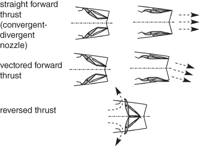
Figure 12.25 Supersonic nozzle area adjustment and thrust vectoring.
12.10 Propeller
Aircraft flying at speeds less than Mach 0.5 are propeller driven, larger aircraft powered by gas turbines and smaller ones by piston engines. More advanced turboprops have pushed flight speed to over Mach 0.7 (Airbus A400). This book deals with the conventional types of propellers operating at flight speed Mach ≤ 0.7. After a brief introduction to the basics of propeller theory, this section concentrates on the engineering aspects of what is required by the aircraft designers. References [13–17] may be consulted for more details. It is recommended to use certified propellers manufactured by well‐known companies.
Propellers are twisted wing like blades that rotate in a plane normal to the aircraft (flight path). They have aerofoil sections that vary from being thickest at the root and to thinnest at the tip chord (Figure 12.26). Thrust generated by propeller is the lift produced by the propeller blades in the flight direction. It acts as a propulsive force and is not meant to lift weight unless the thrust line is vectored. In rotation, the tip experiences the highest tangential velocity. The figure shows associated geometries and symbols used in analysis. The three important angles are blade pitch angle, β, angle subtended by the relative velocity, ϕ, and angle of attack, α = (β – ϕ). Also shown is the effect of coarse and fine blade pitch, β. The definition of propeller pitch, p, is given in Section 12.10.1.
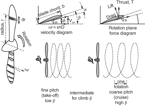
Figure 12.26 Aircraft propeller.
The propeller types are shown in Figure 12.27. There can be anywhere from two blades to as many as seven/eight. Smaller aircraft have two to three blades while bigger ones can have anywhere from four to seven/eight. When the propeller is placed in front of the aircraft, it is called a tractor and when placed at aft, it is called a pusher. The majority of the propellers serve as tractors.
12.10.1 Propeller‐Related Definitions
Industry uses propeller charts, those incorporate some special terminologies. Definitions of the necessary terminologies/parameters are given here:
D = Propeller diameter = 2 × r
n = Revolution per second (rps)
ω = Angular velocity
N = Number of blades
b = Propeller blade width (varies with radius, r)
P = Propeller power
Cp = Power coefficient (not to confuse with pressure coefficient) = P/(ρn3D5)
T = Propeller thrust
CLi = Integrated design lift coefficient (CLd = sectional lift coefficient)
CT = Propeller thrust coefficient = T/(ρn2D4)
β = Blade pitch angle subtended by the blade chord and its rotating plane (also known as geometric pitch)
p = Propeller pitch = no slip distance covered in one rotation = 2πrtanβ (explained previously)
VR = Relative velocity to the blade element = √(V2 + ω2r2) (Blade Mach No: = VR/a)
ϕ = Angle subtended by the relative velocity = tan−1(V/2πnr) or tanϕ = V/πnD. It is the pitch angle of the propeller in flight and is not the same as blade pitch, which is independent of aircraft speed.
α = Angle of attack = (β − ϕ)
J = Advance ratio = V/(nD) = πtanϕ (a non‐dimensional quantity − analogous to α).
AF = Activity factor = (105/16) ![]()
TAF = Total activity factor = N × AF (N is number of blades – it gives an indication of power absorbed).
It is found that at around 0.7r (tapered propeller) to 0.75r (square propeller), the blades give the aerodynamically average value that can be applied uniformly over the entire radius to obtain the propeller performance.
Figure 12.26 shows a two‐bladed propeller along with a blade elemental section, dr, at radius r. The propeller has diameter, D. If ω is the angular velocity then the blade element linear velocity at radius r is ωr = 2πnr = πnD, where n is the number of revolution per unit time. An aircraft with true airspeed of V and with propeller angular velocity of ω, will have blade element moving in a helical path. At any radius, the relative velocity, VR has angle ϕ = tan−1(V/2πnr). At the tip ϕtip = tan−1(V/πnD).
However, irrespective of aircraft speed, the inclination of blade angle from the rotating plane can be seen as solid‐body screw thread inclination and is known as pitch angle, β. The solid‐body screw like linear advancement through one rotation is called propeller pitch, p. The pitch definition has a problem as unlike mechanical screws, the choice of inclination plane is not standardised. It can be the zero‐lift line, which is aerodynamically convenient or the chord line, which is easy to locate or the bottom surface – each plane will give a different pitch. All these planes are interrelated by fixed angles. This book takes the chord line as the reference line for the pitch as shown by blade pitch angle, β, in Figure 12.24. This gives propeller pitch, p = 2πr tanβ.
Since the blade linear velocity ωr varies with radius, its pitch angle needs to be varied as well to make the best use of the blade element aerofoil characteristics. When β is varied in such a way that the pitch is not changed along the radius then the blade has constant pitch. This means that β decreases with increase in r (variation in β is about 40° from root to tip).
Blade angle of attack,
This brings out an analogous non‐dimensional parameter, J = advance ratio = V/(nD) = πtanϕ.
Blade pitch should match with aircraft speed, V, to keep blade angle of attack α to produce best lift. To cope with aircraft speed change, it benefits if the blade is rotated (varying the pitch) about its axis through the hub to maintain favourable α at all speeds. It is then called a variable pitch propeller. Typically, for pitch variation, the propeller is kept at constant rpm with the help of a governor, when it is called a constant speed propeller. Almost all aircraft flying at higher speed will have constant speed variable pitch propeller (when done manually it is β‐controlled). The smaller low speed aircraft are with fixed pitch that would run best at one combination of aircraft speed and propeller rpm. If the fixed pitch is meant for cruise then at takeoff (low aircraft speed and high propeller revolution) the propeller would be less efficient. Typically, aircraft designers would like to have fixed pitch propeller matched for the climb, a condition in between cruise and takeoff to minimised the difference between the two extremes. Obviously, for high speed performance it should match the high speed cruise condition. Figure 12.28 shows the benefit of constant speed variable pitch propeller over the speed range.
The β‐control can extend to reversing of propeller pitch. A full reverse thrust acts as all the benefits of TR describe in Section 12.9. The pitch control can be made to ‘fine‐pitch’ to produce zero thrust when the aircraft is static. This could assist aircraft to wash out speed especially at approach to land.
When the engine fails, that is the system senses insufficient power, the pilot or the automatic sensing device elects to feather the propeller (Figure 12.25). Feathering is changing β to 75–85° (maximum coarse) when propeller slows down to zero rpm – producing net drag/thrust (part of propeller has thrust and the rest drag) to zero.
Windmilling of propeller occurs when the engine has no power and is free to rotate driven by the relative airspeed to the propeller when aircraft is in flight. The β angle is in a fine position.
Installed turboprop thrust is obtained by reducing the thrust by the various loss factors. In addition fuselage factors of fuselage blockage factor fb and excrescence factor fh (see Section 11.16) are to be applied further reducing the thrust level.
12.11 Propeller Theory
The fundamentals of propeller performance start with the idealised consideration of momentum theory. Its practical application in industry is based on subsequent ‘blade element’ theory. Both are presented in this section, followed by the engineering consideration appropriate to the aircraft designers. Industrial practices still use manufacturer supplied propellers and wind tunnel tested generic charts/tables to evaluate performance. There are various forms of propeller charts; the three prevailing ones are (i) the Hamilton Standard [15] (propeller manufacturer) method, (ii) SBAC Standard Method of Performance Estimation [16] and (iii) the NACA (National Advisory Committee for Aeronautics) method [11]. This book uses the Hamilton Standard method used in industry [15]. For designing advanced propellers/propfans to operate at speeds greater than Mach 0.6, CFD is playing an important role to arrive at the best compromise, substantiated by wind tunnel tests. CFD employs more advanced theories, for example, the vortex theory.
12.11.1 Momentum Theory – Actuator Disc
The classical incompressible inviscid momentum theory provides the basis of propeller performance [13]. In the theory, the propeller is represented by a thin actuator disc of area, A, placed normal to free stream velocity, V0. This captures a stream tube within a CV having a front surface sufficiently upstream represented by subscript ‘0’ and at sufficiently downstream by subscript ‘3’ (Figure 12.29). It is assumed that thrust is uniformly distributed over the disc and the tip effects are ignored. Whether the disc is rotating or not is redundant, as flow through it is taken without any rotation. Station numbers just in front and aft of the disc are designated 1 and 2.
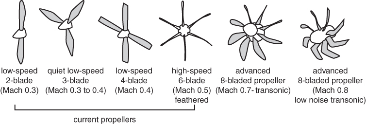
Figure 12.27 Multi‐bladed aircraft propellers (the low noise transonic propeller is taken from unpublished work by Dr R. Cooper at QUB).
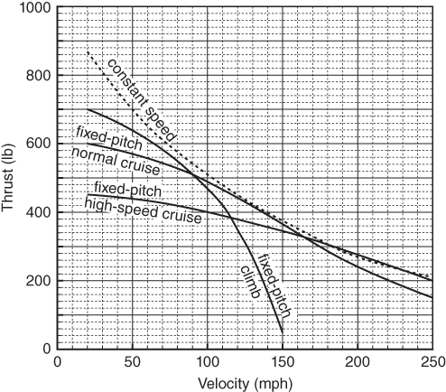
Figure 12.28 Comparison of fixed pitch and constant speed variable pitch propeller (≈200 HP).

Figure 12.29 CV showing the stream tube of the actuator disc.
The impulse given by the disc (propeller) increases the velocity from the free stream value of V0, smoothly accelerating, to V2 behind the disc and continuing to accelerate to V3 (station 3) until the static pressure equals the ambient pressure p0. The pressure and velocity distribution along the stream tube is shown in Figure 12.29. There is a jump of static pressure across the disc (from p1 to p2) but there is no jump in velocity change.
Newton's law gives that the rate of change of momentum is the applied force; in this case it is the thrust, T. Consider station 2 of the stream tube immediately behind the disc producing the thrust. It has MFR, ![]() = ρAdiscV2. The change of velocity is ΔV = (V3 − V0). This is the reactionary thrust experienced at disc through the pressure difference multiplied by its area, A.
= ρAdiscV2. The change of velocity is ΔV = (V3 − V0). This is the reactionary thrust experienced at disc through the pressure difference multiplied by its area, A.
Thrust produced by the disc
Equating, Eq. 12.23 can be rewritten as
The incompressible flow Bernoulli's equation cannot be applied through the disc imparting energy. Instead, two equations are set up, one for conditions ahead of the disc and the other aft of it. Ambient pressure p0 is the same everywhere.
Ahead of the disc,
Aft of the disc,
Subtracting the front relation from the aft relation,
Since there is no jump in velocity across the disc, the last term drops out.
Next substitute the value of (p2 − p1) from Eq. 12.24 into Eq. 12.27.
Note that (V3 − V0) = ΔV when subtracted from Eq. 12.28, it gives 2V3 = 2V2 + ΔV.
Or
It says that half of the added velocity, ΔV/2, is ahead the disc and the rest, ΔV/2, is added aft of the disc.
Using conservation of mass, A3V3 = A1V1, Eq. 12.23 becomes
Using Eqs. 12.29 and 12.30, the thrust Eq. 12.23 can rewritten as
Applying to aircraft, V0 may be seen as aircraft velocity, V, by dropping the subscript ‘0’. Then useful work rate (power, P) done on the aircraft is
For the ideal flow without the tip effects, the mechanical work produced in the system is the power, Pideal, generated to drive the propeller is force (thrust, T) times velocity, V1, at the disc.
Therefore, ideal efficiency,
The real effects will have viscous, propeller tip effects and other installation effects. In other words, to produce the same thrust, the system has to provide more power (in case of piston engine it is seen as Brake Horse Power (BHP) and in case of turboprop as ESHP, where ESHP is the equivalent shaft horse power that converts the residual thrust at the exhaust nozzle to HP, dividing by an empirical factor 2.5. The propulsive efficiency as given in Eq. 12.34 can be written as
This gives,
12.11.2 Blade Element Theory
Practical application of propellers is obtained through blade element theory as given next. Propeller blade cross‐sectional profile has the same functions as that of wing aerofoil, that is, to operate at the best L/D.
Figure 12.26 shows that a blade elemental section, dr, at radius r, is valid for any number of blades at any radius, r. As blades are rotating elements, their properties would vary along the radius.
Figure 12.26 gives the velocity diagram showing an aircraft with a flight speed of V with its propeller rotating at n rps, which would make its blade element advance in a helical manner. VR is the relative velocity to the blade with angle of attack α. Here, β is the propeller pitch angle as defined before. Strictly speaking, each blade rotates in the wake (downwash) of the previous blade, but the current treatment ignores this effect to use propeller charts without appreciable error. Figure 12.26 also gives the force diagram at the blade element in terms of lift, L, and drag, D, that is normal and parallel, respectively, to VR. Then the thrust, dT, and force, dF (producing torque) on the blade element can be easily obtained, by decomposing lift and drag in the direction of flight and in the plane of propeller rotation, respectively. Integrating over the entire blade length (non‐dimensionalised as r/R – an advantage to be applicable to different sizes) would give the thrust, T, and torque producing force, F, by the blade. The root of the hub (with spinner or not) does not produce thrust and integration is normally carried out from 0.2 to the tip, 1.0, in terms of r/R. When multiplied by the number of blades, N, it gives the propeller performance.
Therefore,

And

From the definition, Advance ratio, J = V/(nD).
It can be shown that the thrust to power ratio is best when the blade element works at the highest lift to drag ratio (L/Dmax). It is clear that a fixed pitch blade works best at a particular aircraft speed for the given power rating (rpm) – typically the climb condition is matched for the compromise. It is for this reason, constant speed variable pitch propellers have better performance over a wider aircraft speed range. It is convenient to express thrust and torque in non‐dimensional form as given next. From dimensional analysis (note that the denominator does not have the ½):
In the foot–pound system (FPS),

where σ = ambient density ratio for altitude performance
In FPS system,

where N stands for r.p.m and n stands for r.p.s. The wider is the blade the would be the power absorbed to a point when any further increase would offer diminishing returns in increasing thrust.
A non‐dimensional number defined as
![]() expresses the integrated capacity of the blade element to absorb power. It indicates that increase of blade width outwardly is more effective than at the hub direction.
expresses the integrated capacity of the blade element to absorb power. It indicates that increase of blade width outwardly is more effective than at the hub direction.
![]() expresses the integrated capacity of the total number of blades of a propeller to absorb power.
expresses the integrated capacity of the total number of blades of a propeller to absorb power.
A piston engine or a gas turbine would drive the propeller. Propulsive efficiency, ηp, can be computed by using Eqs. 12.35, 12.39 and 12.44.
Propulsive efficiency

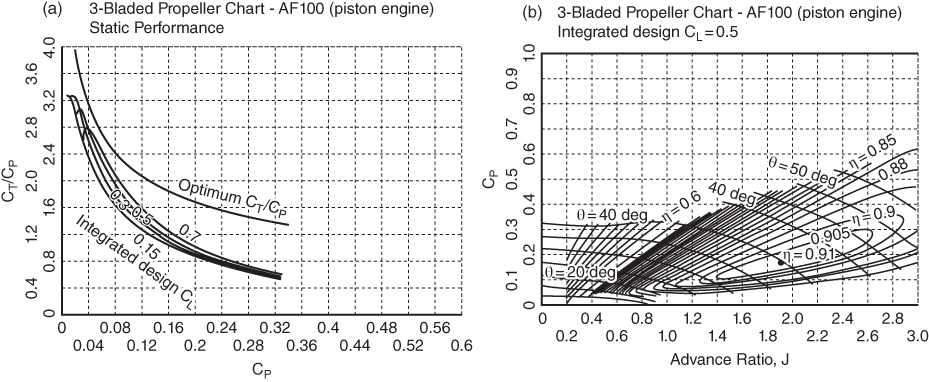
Figure 12.30 Static performance – Three bladed propeller chart – AF100 (for piston engines). (a) Static performance. (b) Propeller performance. (Courtesy of Hamilton Standard – retraced maintaining high fidelity).
Source: Reproduced with permission from Cambridge University Press.

Figure 12.31 Four bladed propeller performance chart, AF180 (for high performance turboprop). (a) Static performance. (b) Propeller performance. (Courtesy of Hamilton Standard – retraced maintaining high fidelity).
Source: Reproduced with permission from Cambridge University Press.

Figure 12.32 Limits of the integrated design CL to avoid compressibility loss. (Courtesy of Hamilton Standard – retraced maintaining high fidelity).
Source: Reproduced with permission from Cambridge University Press.

Figure 12.33 Engine power versus propeller diameter (extracted from [13]).
Source: Reproduced with permission from Cambridge University Press.
12.12 Propeller Performance – Use of Charts, Practical Engineering Applications
The theory determines that geometrically similar propellers can be represented in a single non‐dimensional chart (propeller graph) from combining the previous non‐dimensional parameters such as shown in Figures 12.30 and 12.31 for three bladed propellers and Figures 12.32 and 12.33 for four bladed propellers. A considerable amount of classroom work can be conducted with these graphs. All these graphs and the procedure to estimate propeller performance are taken from [15] courtesy of Hamilton Standard, who kindly permitted use of the graphs in this book. All Hamilton Standard graphs are re‐plotted retaining the maximum fidelity. The reference the gives full range of graphs for other types and has charts for propellers with a higher AF. The charts use the following relations.
Static computation presents a problem, as when V is zero, then ηp = 0. Different sets of graphs are required to obtain take the values of (CT/CP) to compute takeoff thrust as given in Figures 12.30 and 12.31. Finally, Figure 12.32 is meant for selecting the design CL for the propeller to avoid compressibility loss. Thrust for takeoff performance can be obtained from the following equations (FPS): compressibility loss. Thrust for takeoff performance can be obtained from the following equations in FPS:
In flight, thrust:
For static performance (takeoff):
The book does not deal with propeller design. Aircraft designers are to select a propeller offered by the propeller manufacturer, mostly an off‐the‐shelf type, unless specially designed ones are used in consultation with aircraft designers. This section gives the considerations necessary for the aircraft designers to select the appropriate propeller to match the size of engine to produce thrust for the full flight envelope.
The readers may note that the propeller charts for the number of blades only use three variables Cp, β and η (subscript p is dropped). It does not specify propeller diameter and rpm. Therefore, similar propellers with same AF and CLi can use the same chart. Aircraft designers will have to choose AF or CLi based on the critical phase of operation. A propeller selection would seek some compromises as optimised performance for full flight envelope is not possible, especially for fixed pitch propellers.
Of late, certification requirements for noise have affected the issues on compromise, especially for the high performance propeller design. High tip Mach number is detrimental to noise and to reduce it, η is compromised by reducing rpm and/or diameter, hence increased J and/or increased number of blades. Increasing the number of blades would increase cost and weight. Propeller curvature suits transonic operation and helps reduce noise.
Equation 12.22 gives the aerodynamic incidence, that is, the blade angle of attack, α = (β − ϕ), where ϕ is determined from aircraft speed and propeller rpm, that is, a function of J = V/nD. It is desirable to keep α constant along the blade radius to get the best CLi, that is, α is maintained at around 6–8°. The values at 0.7r or 0.75r being used as the reference point – the propeller chart mentions reference radius.
The combination of the designed propeller rpm is matched with its diameter to keep the operation below experiencing compressibility effects at maximum speed at an altitude. A suitable reduction in gear ratio brings the engine rpm down to the desirable propeller rpm. Figure 12.32 is used to obtain the integrated design CL for the combination of the propeller rpm and diameter. The factor ND × (ratio of speed of sound at STD day sea level to the altitude) would establish the integrated design CL. A spinner at the propeller root is recommended to reduce loss. Typically, majority of production propellers have integrated design CL within the range of 0.35–0.6. Figure 12.32 gives the limits of integrated design CL, which should not be exceeded.
The following step‐by‐step observations/information could prove important to progress propeller performance estimation by using the propeller charts given in Figures 12.30–12.32 (Hamilton Standards).
- In this book, the integrated design CL is taken 0.5. Checking of the integrated design CLi using Figure 12.32 is not used.
- Typical blade activity factor, AF is of the following order:
- Low power absorption two to three bladed propellers for home‐built flying = 80 < AF < 90.
- Medium power absorption three to four bladed propellers for piston engines (utility) = 100 < AF < 120.
- High power absorption four bladed and more propellers for turboprops = 140 < AF < 200.
- Keep tip Mach number around 0.85 at cruise and make sure that at takeoff rpm it does exceed the value at the second segment climb speed.
- Typically, for constant speed variable pitch propeller, β is kept low for takeoff, gradually increasing at climb speed, reaching intermediate values at cruise and a high value at the maximum speed. Automatic blade control mechanism design involves specialised engineering.
- Propeller diameter in inches can be coarsely determined by an empirical relation D = K(P)0.25 where K = 22 for two blades, 20 for three blades and 18 for four blades. Power P is the installed power, which is less than the bare engine rating supplied by the engine manufacturer. Figure 12.33 gives the statistics of typical relationship between engine power and propeller diameter. It is a useful graph to deduce the initial size of the propeller empirically.
If n and J are known beforehand, then propeller diameter can be determined using D = 1056 V/(NJ) in the FPS system.
- Maintain at least about 0.5 m (1.6 ft) propeller tip clearance from the ground, for extreme demands this can be slightly reduced. This should take care of nose wheel tyre burst and undercarriage oleo collapse.
- At maximum takeoff static power, thrust developed by propellers is about four times the power.
Continue (in FPS) with propeller performance for static takeoff and in‐flight cruise separately.
Static performance (Figures 12.30 a and 12.31 a)
- Compute the power coefficient, CP = (550 × SHP)/(ρn3D5), where n is in rps. Note ρ for fc.
- From propeller chart find CT/CP.
- Compute static thrust, TS = (CT/CP)(33 000 × SHP)/ND, where N is in rpm.
In‐flight performance (Figures 12.30 b and 12.31 b)
- Compute the advance ratio, J = V/(nD)
- Compute power coefficient, CP = (550 × SHP)/(ρn3D5), where n is in rps.
- From propeller chart find efficiency, ηP.
- Compute thrust, T from ηP = (TV)/(550 × SHP), where V is in ft s−1.
If necessary, off‐the‐shelf propeller blade tips could be slightly chopped off to meet geometrical constraints. Typical penalties are 1% reduction of diameter would affect 0.65% reduction in thrust – for small changes, linear interpolation may be made.
In addition, the fuselage factors blockage factor fb and excrescence factor fh (see Section 12.15) should be applied further reducing the thrust level.
12.12.1 Propeller Performance – Blade Numbers 3 ≤ N ≥ 4
Using these graphs, linear extrapolation could be made for two and five bladed propellers with similar AF and so on. Reference [15] treats the subject in detail with propeller charts for other AF values.
References
- 1. Rolls Royce (1996). The Jet Engine, 5e. Rolls Royce Plc.
- 2. Kundu, A.K. (2010). Aircraft Design. Cambridge University Press.
- 3. Saravanamuttoo, H.I.H., Rogers, G.F.C., Cohen, H., and Straznicky, P.V. (2008). Gas Turbine Theory. Pearson.
- 4. Kundu, A.K., Price, M.A., and Riordan, D. (2016). Theory and Practice of Aircraft Performance, ISBN: 9871119074175. Wiley.
- 5. Mattingly, J.D. (1996). Elements of Gas Turbine Propulsion. McGraw‐Hill.
- 6. Chima, R.V. (2012). Analysis of Buzz in a Supersonic Inlet, NASA/TM—2012‐217612. Cleveland, OH: Glenn Research Centre.
- 7. Oates, G. (1984). Aerothermodynamics of Gas Turbines and Rocket Propulsion. AIAA.
- 8. Swavely, C.E. (1985). Propulsion System Overview, Pratt and Whitney Short Course. Pratt and Whitney.
- 9. Farokhi, S. (1991). Propulsion System Integration Course. University of Kansas.
- 10. Seddon, J. and Goldsmith, E. (1985). Practical Intake Aerodynamic Design. AIAA.
- 11. Gilman, G. (1953). Propeller Performance Charts for Transport Airplane. NACA Technical Note 2966, Langley Aeronautical Laboratory, Langley Field, VA.
- 12. Riordan, D., Class Lecture Notes at QUB, 2003.
- 13. Glauert, H. (1926). Elements of Aerofoil and Airscerw Theory. Cambridge University Press.
- 14. Stinton, D. (1983). The Design of the Airplane. BSP Professional Books.
- 15. Hamilton Standard (1963). Propeller Performance Mannual. Hamilton Standard.
- 16. Society of British Aircraft Constructors (1930). SBAC Standard Method of Performance Estimation. London: SBAC.
- 17. Lan, C.T.E. and Roskam, J. (1981). Aeroplane Aerodynamics and Performance. DAR Corporation.