23
Computational Fluid Dynamics
23.1 Overview
Computational Fluid Dynamics (CFD) is a numerical tool for solving fluid mechanics equations. CFD is a relatively recent development that has grown powerful enough to become an indispensable tool over the last two decades. Originally, it was developed for aeronautical usages, but now pervades all disciplines involving flow phenomena; for example, medical, natural sciences, engineering applications and so on. The built‐in codes of the CFD software are algorithms of numerical solutions to fluid mechanics equations. Flow fields that were previously difficult to solve by analytical means, and in some situations impossible, are now accessible by means of CFD.
Today, the aircraft industry uses CFD during the conceptual study phase and continues with detailed analyses in the next stages after the ‘go‐ahead’ is obtained. There are limitations in getting accurate results, but research continues in academic and industrial circles to improve prediction. This chapter aims to make the newly initiated readers aware of the scope of CFD in configuring aircraft geometry. Those who are already exposed to the subject may skip the chapter. This is not a book on CFD, so this chapter does not present a rigorous mathematical approach but an overview.
CFD is a subject on its own requiring considerable knowledge on fluid mechanics, mathematics and computer science. CFD is introduced late in undergraduate studies in the final years when students have covered the prerequisites. Commercial CFD tools are menu driven and one could become proficient soon enough but to interpret the results thus obtained would require considerable experience in the subject matter.
Making an accurate 3D model of the aircraft with complete aircraft drag (CAD) offers considerable reduction in preprocessing time. The CAD software must have compatible format with CFD to transport the drawing models. Together, CAD and CFD provide a CAE (Computer‐Aided Engineering) approach to paperless electronic design methods.
There are several good commercial CAD and CFD packages in the market place. Nowadays, all engineering schools have CAD and CFD application software. This book refrains from naming any package.
What is to be learnt. The chapter covers the following:
- Section 23.2 Introduces the Concept of CFD
- Section 23.3 Introduces the Current Status of CFD
- Section 23.4 Presents an Approach Road and Considerations for CFD Analysis
- Section 23.5 Presents Some Case Studies
- Section 23.6 Suggests the Extent of Classroom Work to be Undertaken
- Section 23.7 Gives a Summary of Discussions
Classwork content. There is no classroom work on CFD in the first term. However, it is recommended that CFD studies should be undertaken in the second term after the reader is formally introduced to the subject. It would require appropriate supervision to initiate the task and analyse results. Any CFD work is separated from the scope of what this book can offer. This chapter is only to give the newly initiated a taste of aircraft design work.
23.2 Introduction
Throughout the book, it is shown that the aerodynamic parameters of lift, drag and moments associated with aircraft moving through air are of vital importance. An accurate assessment of these parameters is the goal of the aircraft designers.
Mathematically, lift, drag, and moment of the body can be obtained from integrating the pressure and shear stress field around the aircraft computed from the governing conservation equations (differential or integral forms) of mass, momentum and energy along with the equation of state for the medium of air. Up until the 1970s, wind‐tunnel tests were the only way to get the best results to obtain these parameters in various aircraft attitudes representing what can be encountered within the full flight envelope. Semi‐empirical formulae generated from vast amounts of test results, backed up by theory, give a good starting point for any conceptual study.
Numerical methods for solving differential equations have been prevailing for some time. Navier–Stokes equations give an accurate representation of the flow field in and around the body under study. But solving these equations for 3D shapes in compressible flow was difficult, if not sometimes impossible. Mathematicians devised methods to discretise differential equations into algebraic form which are solvable even for the difficult non‐linear partial differential equations. During the early 1970s, CFD results of simple 2D bodies in inviscid flow were demonstrated to be comparable with wind tunnel test results and analytical solutions.
Industry and national laboratories saw its potential and progressed with in‐house research, and in some cases was able to understand complex flow phenomena hitherto unknown. Subsequently, it proliferated into academies and rapid advancement was achieved for the solution techniques. Over time, the methodologies kept improving. The latest techniques discretise the flow field into finite volumes in various sizes (smaller where the fluid properties have steeper variation) matching the wetted surface of the object, which also needs to be divided into cells. The cells do not overlap the adjoining volumes but mesh seamlessly. The mathematical formulation of the small volumes can now be treated algebraically to compute the flux of the conserved properties between the neighbouring cells. Discrete steps of algebraic equations are not calculations of limiting values at a point; therefore, error creeps into the numerical solution. Mathematicians are aware of the problem and struggle with better techniques in making the algorithm minimise the error. This numerical method of solving fluid dynamic problems became computation intensive, requiring computers to tackle a large number of cells; their numbers could run into several millions. The solution technique is thus known as Computational Fluid Dynamics.
The other problem in the 1970s was the inadequacy of the computing power available to tackle the domain comprising of a large number of cells and handle error functions. As computer power increased along with superior algorithms, CFD capability started to become applicable to industry. Today, CFD is a mature method and is well supported by advanced computing power. CFD started in industry and now has finally become an indispensable tool for the industry and research establishments.
One of the difficult areas of CFD simulation lies in turbulence modelling. Over the last two decades, computations of 3D Reynolds‐average Navier–Stokes (RANS) equations for complete aircraft configurations became routine. Reference [1] summarises the latest trends in turbulence modelling. A large number of credible application software packages have emerged on the market, some catering for special purpose applications.
As discussed, drag predictions around the design point have improved to become relatively reliable, comparable to WT results (without incurring the cost of testing at high Reynolds number). As discussed, drag predictions around the design point are reliable, comparable to wind‐tunnel test results (without incurring the cost of testing at high Reynolds number) stall point, unsteady phenomena, for example, buffet, high angle of attack and separated flows, are not so reliably predicted. CFD still has its limitations. Drag is a viscous dependent phenomenon; inclusion of viscous terms makes the governing equations very complex requiring intensive computational time. Capturing all the elements contributing to drag of a full aircraft is a daunting task – its full representation is yet to achieve credibility in the industrial usages. It is not yet possible to get accurate drag prediction using CFD without manipulating input data based on the designer's experience. However, once set up for the solution, the incremental magnitudes of aerodynamic parameters of a perturbed geometry are well represented in CFD. It is a very useful tool to obtain accurate incremental values of a perturbation geometry from a baseline aircraft configuration with known aerodynamic parameters. It offers a capability to make parametric optimisation to a certain degree (see the next section).
23.3 Current Status
Chapman [2] in his classic review (1979) advocates the indispensability of CFD, as the computers start showing the promise of overtaking experiments as a principal source of detailed information on design. His view is now regarded as an overoptimistic estimate. CFD capabilities can compliment experiments. He assigned the following three main reasons for his conclusion:
- Experiments cannot represent the real flight envelope (Re, temperature etc.) and are limited by flow non‐uniformity, wall effects and transient dependent separation.
- Very high energy (cost) associated with large tunnels.
- CFD is faster and cheaper than experiments to obtain some valuable insight at an initial stage.
He showed the chronology of progress to be in four stages, starting from the late 1960s solving linear potential flow equations, to arriving at a stage when the non‐linear Navier–Stokes equations can be tackled.
In his recent paper, Chapman [3] again reviewed the rapid progress achieved in the last decade. With a better understanding of turbulence and with advances in computer technology, both in hardware and software development, researchers have successfully generated aerodynamic results that were impossible to obtain until then.
The latest review by Roache [4] demonstrates that considerable progress has been achieved in CFD, but the promise is still far from being fulfilled in estimating CAD. AGARD report AR256 [5] gives technical status review on drag prediction and analysis from a CFD point of view. In that report, Schmidt categorically stated that ‘consistent and accurate prediction of absolute drag for aircraft configuration is currently beyond CFD reach …’. Many researchers were also of the same opinion, stating that the CFD flow modelling was found to be lacking in ‘certain respects’. Both agreed that the current state‐of‐the‐art in CFD is still a useful tool at the conceptual stages of design for comparison of shapes and for diagnostic purposes.
An essential route to establish the robustness of any CFD comes through the success of the conceptual model code verification and validation. Roache [4] uses the semantics of ‘verification’ as solving the equations correctly and ‘validation’ as solving the correct equations. The process of benchmarking (code to code comparison) results in the selection of the best value for money software, not necessarily the best software on the market.
Experimental results are used to validate and calibrate CFD codes. Various degrees of success have been had in case to case studies. Melnik [6] showed that the current CFD status in aircraft drag prediction of a subsonic jet transport type aircraft wing on a simple circular cross section fuselage had mixed success, as shown in Figure 23.1. Some correlation was achieved after considerable ‘tweaking’ of the results. The results using these methods are not certifiable because of considerable ‘grey’ areas.

Figure 23.1 CFD simulation of wing‐body drag polar [6]. Reproduced with permission from Cambridge Unversity Press.
Currently, industry uses the CFD as a tool for flow field analysis, wherever possible to estimate drag in inviscid flow, for example, induced drag and wave drag, but not used for CAD estimation. In industry, CFD appears as a general purpose tool to simulate flow around objects for qualitative studies and diagnostic purposes. For the design point, design of high‐lift system, full RANS simulations are used.
It is difficult to capture large number of ‘manufacturing defects’ (e.g. steps, gaps, waviness etc., arising from surface smoothness requirements) over the full aircraft. CFD flow field analysis of simple geometries for benchmark work has been carried out, for example on large backward facing steps. One such example is Thangam et al. [7] who describe a detailed study of flow past backward steps to understand turbulence modelling (κ‐ɛ). This type of work does not represent the problems associated with the small geometries of excrescence effects nor can they guarantee accuracy. Another example is Berman's [8] work on a large rearward facing step, but this is not representative of the dimensions of excrescence.
Assessment of excrescence drag using CFD needs a better understanding of the structure of the boundary layer in turbulent flow. While there exists voluminous literature on CFD code generation and qualitative assessment of pressure field, no work has been cited about estimating parasite drag of excrescences. As modern CFD software becomes more capable, it may become possible to predict excrescence drag simulating real cases with double curvature in compressible flow with or without shocks or separation.
Reference [9] includes verification of excrescence drag on a flat plate in the absence of a pressure gradient to estimate the excrescence drag on a 2D aerofoil in pressure gradient. The study on an aerofoil [10] may be seen as a precursor to examine the scope for CFD estimates of excrescence drag on the generic 3D aerofoil configuration.
This review provides some earlier CFD studies conducted during the twentieth century. Since then, considerable progress has been made in refining programme algorithms to improve accuracy and rapid improvement at lower cost has made CFD an essential tool for flow analyses in industries and academies.
Based on the Boeing Company's endeavours with CFD, Forrester et al. [11] summarise progress made in the last three decades, as quoted here:
CFD will continue to see an ever‐increasing role in the aircraft development process as long as it continues to add value to the product from the customer's point of view. CFD has improved the quality of aerodynamic design, but has not yet had much effect on the rest of the overall airplane development process. CFD is now becoming more interdisciplinary, helping provide closer ties between aerodynamics, structures, propulsion and flight controls. This will be the key to more concurrent engineering, in which various disciplines will be able to work more in parallel rather than in the sequential manner as is today's practice. The savings due to reduced development flow time can be enormous!
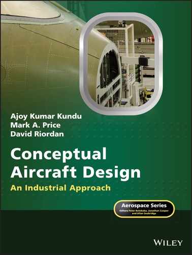
Jameson clearly sums up in [1] in his review of the past and the present of CFD activities then projecting the direction of future work. Figure 23.2 shows the CFD contribution to the Airbus380 aircraft. It corroborates the statement made in [1] that ‘CFD has improved the quality of aerodynamic design, but has not yet had much effect on the rest of the overall airplane development process’.
Figure 23.2 CFD contribution to Airbus380 aircraft [1].
23.4 Approach Road to CFD Analyses
CFD analysis requires preprocessing of the geometric model before computation can start. It comprises of creating an acceptable geometry (2D or 3D) amenable to analysis (say there is no hole for fluid to leak through). A preprocessing package comes with its own CAD to create geometry, specifically suited for a seamless entry to the solver for computation. However, a considerable amount of labour can be saved if the aircraft geometry already created in CAD can be used in CFD. This is possible if care has been taken in creating a geometry that is transportable to CFD preprocessing environments.
The next task is to lay a grid on the geometry for CFD to work on small numbers of cells at a time until the entire domain is tackled. The surface grids should be intelligently laid to capture details where there is large local geometric variation, normally at the junction of two bodies and where there is steep curvature. The next step would be to generate cells in the domain of application, which could be a large flow field space around the body. Evidently, at the far field, the variation in the flow field between the cells is low and therefore could be made larger. The preprocessor is menu driven and gives the options for various kinds of grid generation to select from. Grids must meet the boundary conditions as the physics dictate. Figure 23.3 gives a good example of aircraft geometry (simplified by excluding empennage and nacelle) with structured grids on it and a section of the environment to be analysed. Only one half of the aircraft, because it is symmetrical on the vertical plane, needs to be analysed – the other half is the mirror image.

Figure 23.3 Wing‐fuselage geometry with meshing. (a) On the surface (Courtesy Aerospatiale). (b) On the surface and in the space [12] (denser close to the surface) From Dr. Raymond Devine's PhD work at QUB.
Figure 23.3b is another example of 3D meshing on a complete aircraft with the nacelle included and in space.
After grid generation in the preprocessor, the model is then introduced into the flow solver, which is also menu driven. The options in the solver are specific and the user must know what to apply. After the solver, a run occurs to compute results (run‐time depends on the geometry, type of grid and solver options as well as the computing power).
The results can be examined in many different ways in a post‐processor. The important ones on an aircraft body are the Cp distribution, the temperature distribution, streamlines and velocity vectors and so on. The Cp distribution and the temperature distribution are shown in grades of colour representing bands of ranges. Figure 23.4b is a grey scale version of the colour distribution and Figures 23.4a depict the flow field streamlines. The results can also be obtained numerically in tabular form. It is clear now that the readers must have the background and be familiar with the CFD software package. For the newly initiated, it should be conducted under supervision.
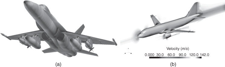
Figure 23.4 CFD post‐processor visualisation (a) Pressure distribution (Courtesy NASA). (b) Velocity Streamline patterns.
Figure 23.5 CFD analysis of a 2‐D aerofoil. (a) Preprocessor showing adaptive grid. (b) Post‐processor showing Mach isolines. (c) In spectrum. Reproduced with permission from Cambridge University Press.
Here is a summary of the approach to CFD:
In the Preprocessor (Menu Driven)
- Step 1. Create geometry – the 3D geometry of the aircraft
- Step 2. Generate grid on the body surface and in the domain of application.
Match to the boundary conditions.
In the Flow Solver (Menu Driven)
- Step 3. Bring the preprocessed geometry and volume mesh into the solver.
Set boundary and initial conditions. Make appropriate choices for the solver.
Run the solver.
Check results and refine (iterate) if necessary (including the grid pattern).
In the Post‐Processor (Menu Driven)
- Step 4. The result thus obtained from the solver can now be viewed in the solver.
Select the display format.
- Step 5. Analyse results.
- Step 6. For a new set up, verify and validate results.
The results can be presented in many ways, for example, Cp distribution, pressure contours, streamlines, velocity patterns, CL, CD, L/D or parameters that can be defined by the user. It can depict shock patterns, location, separation and so on, similar to what wind tunnels can do with flow visualisation. These give an insight to the aerodynamics designers need to improve a design for say, best L/D, best aerodynamic moments, compromise shapes to facilitate production and so on.
The results may need tweaking for which iterations would be necessary starting from Step 2 and/or Step 3.
23.5 Some Case Studies
This section includes some elementary examples of some case studies starting with 2D cases as shown in Figure 23.5. The first diagram represents an aerofoil with the grid layout shown.
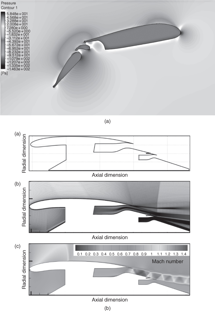
Figure 23.6 CFD flow analyses case studies. (a) High‐lift device. (b) Nacelle grids for internal and external flow analysis.
The domain of analysis is large with anisotropic adaptive grid (Figure 23.5a), which is dense close to the leading edge and trailing edge matching the surface grids, and where there are shocks present. Once the solver is run, the result can be seen in the post‐processor showing the Mach number iso‐lines (Figure 23.5b). At another run with a different set up, the result is shown in colour spectrum (grey scale version in Figure 23.5c).
CFD analysis of a component should prove relatively easy but flow with internal and external flow through nacelle can be a difficult case. The example is of high‐lift device analyses as shown in Figure 23.6a. Nacelle grids for internal and external flow analysis are shown in Figure 23.6b.
While CFD studies around aerofoils exist, flow field analysis around nacelles is rare. Chen et al. [15] present a flow field analysis over a symmetric isolated nacelle using a Euler solver (Figure 23.7). Subsequent studies by Uanishi et al. [16] show confirmation of velocity field obtained by Chen. No work has been located for velocity fields over nacelle using Navier–Stokes solvers.
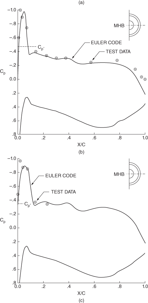
Figure 23.7 CFD results of a nacelle by Chen et al. [16]. (a) Nacelle geometry. Reproduced with permission from Cambridge Unversity Press. Comparisons of Cp at different M∞ values along the maximum half breadth. (b) M∞ = 0.6 (c) M∞ 0.84. Reproduced with permission from Cambridge Unversity Press.
In a very fine recent analysis [17], it is stated that
… the observed scatter in the absolute CFD‐based drag estimates is still larger than the desired single drag count error margin that is defined for drag prediction work. Yet, the majority of activities conducted during an aircraft development programme are incremental in nature, that is, testing/computing a number of options and looking for the best relative performance.
23.6 Hierarchy of CFD Simulation Methods
A hierarchy of CFD simulation methods exists in which they are classified according to the physics they are capable of modelling. At the top of the hierarchy are Direct Numerical Simulations (DNSs) simulating time‐dependent turbulent flows, capturing the dynamics of the whole temporal and spatial spectrum of eddy sizes. This requires grids and time steps that are finer than the length and time scales at which turbulent energy is dissipated. Low diffusion numerical schemes are necessary. It is very useful for supplementing experimental data and aiding the development of turbulence models, but prohibitively expensive at flight Reynolds numbers. It is not used in the design process. Currently, it is the most sophisticated method.
- Large Eddy Simulation (LES) technique. LES takes advantage of the fact that the smallest, dissipative eddies are isotropic. These can be efficiently modelled using simple sub‐grid scale models. Meanwhile, the dynamics of the larger eddies, which are anisotropic in nature, is simulated using a grid and time step sufficiently fine to resolve them accurately. The method is, therefore, applicable to flows at relatively large Reynolds numbers, but is still expensive to use as an engineering design tool.
- Detached Eddy Simulation (DES) technique. DES can be considered a halfway house between LES and RANS. The method employs a RANS turbulence model (next in the list) for near‐wall regions of the flow and a LES‐like model away from the wall. The method was first proposed by Spalart et al. in 1997 and is still the subject of research. It may become a standard engineering tool, but at present it is unlikely to be an element of the conceptual and preliminary design toolkits.
- Reynolds‐averaged Navier–Stokes equations (RANS) technique. The time‐dependence of turbulent fluctuations is averaged out to form the RANS equations. This results in the appearance of so‐called Reynolds stresses in the equations, and the problem of modelling these (turbulence modelling) arises. There are many turbulence models, but each one falls prey to the fact that turbulence is flow‐dependent; consequently, no turbulence model can be generally applicable, and the CFD practitioner must be cognisant of the strengths and failings of the models he/she employs. Nonetheless, RANS does allow relatively inexpensive modelling of complex flows, and when allied to a suitable optimisation method, can be a powerful tool for design synthesis.
- Euler equations technique. The Euler equations are obtained when the viscous terms are dropped from the Navier–Stokes equations. This allows fast predictions of pressure distributions and can be usefully employed at the preliminary design stage. Viscous effects can be included by integrating boundary layer methods, and displacing the surface of the aerofoil/wing/aircraft by an amount equal to the local boundary layer displacement thickness.
- Full potential flow equations. The full potential flow equations assume that the flow is irrotational. Compressible flows can be modelled, but the ‘shocks’ that are predicted are isentropic. The method is now quite dated, but can provide very rapid information about pressure distributions, and can, like the Euler equations, be integrated with a boundary layer method.
- Panel method. This is simplest of all numerical methods for predicting flow about aircraft and may be seen as a precursor for CFD. The surface of the aircraft is covered with panels, each one a source or sink and some of them, for example, those on lifting surfaces, assigned a bound vortex (with its associated trailing vortex system). The strengths of the sources and bound vortices are initially unknown, but can be determined through the application of the boundary conditions, for example, flow tangency at solid surfaces.
Descending through the hierarchy, the methods provide less and less physical fidelity, but require less and less computational effort. It is conceivable that the panel methods, full potential flow equations, Euler equations and RANS methods could be used in an undergraduate aircraft design project (as a separate task), though not at the conceptual design stage. These methods would give a qualitative pressure distribution pattern to help shape the geometrical details. Whatever method is used, the issue of grid generation must be addressed: more time will be spent on the generation of a suitable mesh than on the prediction of the flow.
A 3D model created in CAD would prove useful at this stage. There should be some planning to prepare the 3D model in CAD in such a way that Boolean operations can build the aircraft model from isolated components, while retaining the isolated components for separate analysis. The wing‐fuselage analysis would give tailless pitching moment data, which is useful information to design aircraft horizontal tail and its relative setting with respect to the fuselage to minimise trim drag.
CFD results could be compared with the results obtained through using the semi‐empirical relationship, for example, drag (Chapter 9). Generally, it is considered that semi‐empirical drag results give good accuracy validated on many aircraft consistent over a long time of usage.
Figure 9.9 presents the wave drag, CDw for the Mach number. CFD gives a fine opportunity to generate a more accurate viscous independent wave drag versus Mach number. Once the CFD results are available then the data in Figure 9.9 may be replaced and hence a further iteration on the drag polar of the aircraft is obtained. CFD is also a good place to generate ΔCDp values and can be used for comparison. In general, CFD generated ΔCDp values should give good values provided the CFD is set up properly.
If the CFD results come within 10% of the results obtained using semi‐empirical relations then it may be considered good. Some tweaking of the CFD runs should improve the result – this is where experience helps. Once the CFD is set up to yield good results then it would prove useful to improve and/or modify aircraft configuration through extensive sensitivity studies. The spectrum plots in colour would show hot spots contributing to drag (local shocks, separation etc). These details cannot be seen so easily by other means. Designers can then follow through repairing the hot spots to reduce drag. The opportunities are unique to CFD making it an indispensable tool to optimise configuration for minimum drag.
If there is a large difference between CFD and semi‐empirical results then it should be investigated properly.
23.7 Summary of Discussions
CFD simulation is a digital/numerical approach to design incorporated in the virtual design process using computers. The current status is adequate enough to make comparative analysis at low cost and time and therefore must be applied in the early conceptual design phase as soon as a CAD 3D model drawing is available. The development of CFD is not necessarily driven by the aerodynamic considerations by itself but driven by the requirements for having a tool to design a better product for lower cost and less time.
CFD continues to develop with greater computing power at lower costs and less time along with the advances made in the algorithm to tackle solutions offering considerable ease and automation for the users to benefit from. While researchers have achieved a good degree of accuracy in drag prediction for a clean aircraft configuration, its generalised application by engineering users is yet to achieve consistency in the results. Verification and validation of the results from CFD analysis are essential for substantiation and the state‐of‐the‐art is still under scrutiny and continuing to develop. Verification of new CFD software comes before validation and together they involve a protracted process in which research continues.
CFD analyses supplement wind‐tunnel tests and they work together to reduce the time and cost frame of a new aircraft project. CFD analyses precedes wind‐tunnel tests. The arguments or considerations (pros and cons) of each type of study is briefly described next.
23.7.1 CFD Analyses
- Cons. Results are sensitive to the type of software used and how the preprocessor (e.g. grids) is prepared. Errors and discrepancies involved are hard to explain. Analyses of CFD results considerable design experience to correlate with real situation. CFD requires test data (wind tunnel/flight tests) to verify and validate post processed output result. As mentioned before.
- Pros. CFD can provide a reasonable understanding of the flow physics quite fast and at low cost. It can select a better configuration from a large number of parametrically varied cases to consider so narrow down the choice, even when as quoted above (Section 23.3) that ‘has not yet had much effect on the rest of the overall airplane development process’. Accurate modelling of turbulence is under developmental process. Yet CFD analyses can narrow down the choice to reduce the number of wind tunnel tests required. The number of many perturbed wind tunnel aircraft models required to make parametric optimisation is considerably reduced.
23.7.2 Wind Tunnel Tests
- Cons. Expensive and time consuming.
- Pros. Test results are realistic, quantifiable as close it can to the actual aircraft capability and errors can be assessed. This assures aircraft capability to plan flight test in a safer manner. CFD helps to minimise the number tests required to get complete information a sought at that phase.
23.7.3 Flight Tests
- Flight test culminates the design process in the progressive manner starting with CFD analyses at the conceptual design phase when not much information is available. Flight tests are the final result of the aircraft capability in reality and substantiated for certification.
- Industry as a conservative user needs to ensure fidelity of the design. However, CFD is capable of comparing designs to recognise the better ones even if its absolute values remain under scrutiny. This capability brings out the best compromise at an early phase of the project at low cost and time avoiding subsequent costly modifications of aircraft configuration, that is, it gives the opportunity to make the design right‐first‐time. The design is subsequently tested in a wind tunnel for substantiation. Today, this approach is a matured one requiring little change to the design after the final flight test results.
- Industrial effort in CFD is extensive and is not suitable study for an undergraduate course. However, classroom work can follow the industrial approach tackling smaller problems such as those given in Section 23.5.
References
- 1. Jameson, A. (2015). Computational Fluid Dynamics – Past, Present and Future. USA: Stanford University.
- 2. Chapman, D. (1979). Computational aerodynamics development and outlook. AIAA Journal.
- 3. Chapman, D. (1992). A perspective on Aerospace CFD. Aerospace America.
- 4. Roache, P.J. (1998). Verification and Validation in Computational Science and Engineering. ISBN: 0‐913478‐08‐3.
- 5. AGARD AR 256. (1989). Technical status review on drag prediction and analysis from computational fluid dynamics: State‐of‐the‐art.
- 6. Melnik, R. E., Siclari, M. J., and Marconi, F. (1995). An overview of a recent industry effort at CFD Code Validation. AIAA pare 95–2229, 26th AIAA Fluid Dynamic Conference.
- 7. Thangam, S. and Speziale, C.G. (1992). Turbulent flow past a backward‐facing step: a critical evaluation of two‐equation method. AIAA Journal 30 (5).
- 8. Berman, H, Anderson, J. D. and Drummond, P. (1982). A numerical solution of the supersonic flow over a rearward‐facing step with transverse non‐reacting hydrogen injection. AIAA paper No: 82–1002.
- 9. Kundu, A. K. and Morris, W. H. (1997). Effect of manufacturing tolerances on aircraft aerodynamics and cost. WMC 97 Conference paper No: 711–003.
- 10. Cook, T. A. (1971). The effects of ridge excrescences and trailing edge control gaps on two‐dimensional aerofoil characteristics. ARC R&M No: 3698.
- 11. Forrester, T., Johnson, E.N., Tinoco, N., and Jong, Y. (2005). Boeing Commercial Airplanes, 1115–1151. Seattle: Washington Computers and Fluids 34.
- 12. Computational Fluid Dynamics is the Future. Website, http://cfd2012.com/wings.html (accessed June 2018).
- 13. Arafat, A. Website, Compressible aerodynamics of commercial aircraft' simulation project. Available at https://www.simscale.com/forum/t/compressible‐aerodynamics‐of‐commercial‐aircraft‐simulation‐project‐by‐ali‐arafat/1142/2 (accessed June 2018).
- 14. Goulas, I., Stankowski, T., Otter, J., and MacManus, D. (2016). Aerodynamic Design of Separate‐Jet Exhausts for Future Civil Aero‐Engines ‐ Part I: Parametric Geometry Definition and Computational Fluid Dynamic Approach. Paper No: GTP‐15‐1538, Journal of Engineering for Gas Turbines and Power, ASME, March 15, 2016.
- 15. Chen, H. C., Yu, N.J., Rubbert, P. E. and Jameson, A. (1983). Flow simulation of general nacelle configurations using Euler equations. Conference paper No: AIAA 83–0539.
- 16. Uanishi, K., Pearson, N. S, Lahnig, T. R. and Leon, R. M. (1991). CFD based 3‐D turbofan nacelle design system. AIAA Paper No: A91–16278.
- 17. Laban, M. (2003). Application of CFD to drag analysis and validation with wind tunnel Data. Nationaal Lucht‐en Ruimtevaartlaboratorium. Lecture Series, Von Karman Institute for Fluid Dynamics.