14
Aircraft Sizing, Engine Matching and Variant Derivatives
14.1 Overview
Chapter 8 configured a preliminary geometry of a new aircraft based on the laid out specifications. It started with the estimated maximum takeoff mass (MTOM), wing reference area, SW, and engine size from the available statistics of past designs for the class of aircraft. The fuselage geometry was determined to accommodate what it has to house, for example, in case of civilian aircraft, the number of passengers and in the case of military designs, the engine, fuel volume, equipment and so on. Chapter 9 laid out the undercarriage based on an estimated aircraft aft centre of gravity (CG) position. Empennage size is linked with wing SW and where it is placed in relation to it. With these preliminary aircraft component geometries, a proper estimate of aircraft MTOM and CG position was evaluated in Chapter 10. At this point, if the estimated MTOM differed (very likely) from the guessed MTOM, the first iteration is required to reconfigure the aircraft primarily affecting the SW. Together, this presented a ‘concept definition’ of the new aircraft project at the Phase I stage of conceptual design study.
The next step in the conceptual design study is the size of the aircraft with the proper reference wing area SW with a matched engine to be more precise than a guesstimate taken from statistics.
The aircraft sizing and engine matching routine is a necessary procedure for a new aircraft project starting early at the conceptual design stage. This is to freeze the aircraft configuration to concept finalisation to obtain the project go‐ahead. The exercise requires aircraft performance analyses for which aircraft drag characteristics should be known along with engine performance details to provide the exact power required. Aircraft drag polar and engine performance capability for the full operational envelope are generated in Chapters 11 and 13, respectively.
The sizing and engine matching exercise are carried out in this chapter to ensure the best configuration to satisfy customer specifications and the mandatory airworthiness requirements. The procedure does not require full aircraft performance analyses. Only the airworthiness requirements and customer specification requirements are checked out in a parametric search as will be shown. Aircraft sizing and engine matching exercise does not guarantee overall aircraft performance in detail but make certain that the new project is capable of meeting the necessary specifications and requirements. After freezing the design to the final configuration through a formal sizing and engine matching exercise, a complete aircraft performance is carried out in Chapter 15. Aircraft performance of the aircraft in extensive details is carried in [1, 2] and may be used as companion books, if required.
It was mentioned earlier that a family of derivative variant aircraft can be offered to cover a wider market at a lower development cost by retaining component commonality. The possible variants for the worked‐out examples are offered in Chapter 8. Typically for civil aircraft, the variant designs (at least three in the family) are offered with the baseline aircraft is in the middle plus one bigger growth version and one smaller shrunk version retaining maximum component commonality within all three designs.
Therefore, the objective of the sizing and engine matching exercise is to fine‐tune the baseline configuration in the middle is to present a ‘satisfactory’ configuration offering a family of variant designs. None may be the optimum but together they offer the best fit to satisfy many customers (i.e. operators) and to encompass a wide range of payload‐range requirements, resulting in increased sales and profitability. To repeat, optimisation of individual goals through separate design considerations may prove counterproductive and usually prevent the overall (global) optimisation of ownership cost. Designers' experience is vital to success; it has to be used.
This chapter proposes a formal methodology to reach an appropriate concept definition of the new aircraft project offering variant designs by refining the concept definition based on statistics. At this stage, another iteration will be required if the sized wing reference area, SW and engine size are different from the initial values taken from statistics. The iteration goes through the full cycle from Chapters 8–11. The newly initiated will invariably face it and must not neglect the iteration.
The two classic important parameters – (i) wing loading (W/SW) and (ii) thrust loading (TSLS/W) are instrumental in the methodology for aircraft sizing and engine matching. The formal methodology seeks to obtain the sized W/SW and TSLS/W for the baseline aircraft. These two loadings alone provide sufficient information to conceive aircraft configuration in a preferred aircraft size with a family of variant designs. Empennage size is governed by wing size and location of the CG. This study is possibly the most important aspect in the development of an aircraft, finalising the external geometry.
14.1.1 Summary
Because the preliminary configuration is based on past experience and statistics, an iterative procedure ensues to fine‐tune the aircraft converging into the correct size of the wing reference area for a family of variant aircraft designs and matched engines. Wallace [3] provides an excellent presentation on the subject and Loftin [4] provides an aircraft sizing exercise in detail.
This chapter includes the following sections:
- Section : Introduction
- Section : Theory
- Section : Coursework Exercises for Civil Aircraft (Bizjet)
- Section : Sizing Analysis and Variant Designs: Civil Aircraft (Bizjet)
- Section : Coursework Exercises for Military Aircraft (AJT)
- Section : Sizing analysis and Variant Designs: Military Aircraft (AJT)
- Section : Aircraft Sizing Studies and Sensitivity Analyses
- Section : Discussions
Coursework content. This is an important chapter. Readers are to compute the parameters that establish the criteria for aircraft sizing and engine matching. The final size is unlikely to be identical to the preliminary configuration obtained in Chapter 8 using statistics of past designs. It is recommended that the readers make use of spreadsheets to carry out the iterations.
14.2 Introduction
In a systematic manner, the conception of a new aircraft progresses from generating market specifications followed by the preliminary candidate configurations that rely on statistical data of past designs in order to arrive at a baseline design, selected from several candidate configurations. In this chapter, the baseline design of an aircraft is formally sized with a matched engine (or engines) along with the family of variants to finalise the configuration (i.e. external geometry and MTOM. An example from each class of civil (i.e. the Bizjet) and military (i.e. the Advanced Jet Trainer, AJT) aircraft are used to substantiate the methodology. The turboprop trainer (TPT) sizing follows the same routine as done for the AJT and is left to the readers to carry out.
14.2.1 Civil Aircraft
Based on circa 2000 fuel prices, the aircraft cost contributes to the direct operating cost (DOC) three to four times the contribution made by the fuel cost. It is not cost effective for aircraft manufacturers to offer custom‐made new designs to each operator with varying payload‐range requirements. Therefore, aircraft manufacturers offer aircraft in a family of variant designs. This approach maintains maximum component commonality within the family to reduce development costs and is reflected in aircraft unit‐cost savings. In turn, it eases the amortisation of nonrecurring development costs, as sales increase. It is therefore important for the aircraft sizing exercise to ensure that the variant designs are least penalised to maintain commonality of components. This is what is meant by producing satisfying robust designs; these are not necessarily the optimum designs. Sophisticated multi‐disciplinary optimisation (MDO) is not easily amenable to ready use. The industries also use parametric search for a satisfying robust design.
To generate a family of variant civil aircraft designs, the tendency is to retain the wing and empennage as almost unchanged while plugging and unplugging the constant fuselage to cope with varying payload capacities. Typically, the baseline aircraft remains as the middle design. The smaller aircraft results in a wing that is larger than necessary, providing better field performances (i.e. takeoff and landing); however, the cruise performance is slightly penalised. Conversely, larger aircraft have smaller wings that improve the cruise performance; the shortfall in takeoff is overcome by providing a higher thrust‐to‐weight ratio (TSLS/W) and possibly with better high‐lift devices, both of which incur additional costs. The baseline aircraft approach speed, Vapp, initially is kept low enough so that the growth of Vapp for the larger aircraft is kept within the specifications. Of late, high investment with advanced composite wing‐manufacturing method is in a better position to produce adjusted wing sizes for each variant (large aircraft) in a cost effective manner, offering improved economics in the long run. However, for some time to come, metal wing construction is to continue with minimum changes in wing size to maximise component commonality.
Matched engines are also used in a family to meet the variation of thrust (or power) requirements for the aircraft variants. The sized engines are bought‐out items supplied by engine manufacturers. Aircraft designers stay in constant communication with engine designers in order to arrive at the family of engines required. A thrust variation of up to ±30% from the baseline engine is typically sufficient for larger and smaller aircraft variants from the baseline. Engine designers can produce scalable variants from a proven core gas‐generator module of the engine – these scalable projected engines are known loosely as rubberised engines. The thrust variation of a rubberised engine does not affect the external dimensions of an engine (typically, the bare engine length and diameter change only around ±2%). This book uses an unchanged nacelle external dimension for the family variants, although there is some difference in weight for the different engine thrusts. The generic methodology presented in this chapter is the basis for the sizing and matching practice.
14.2.2 Military Aircraft
It follows the same procedure as in the civil aircraft methodology except that the specifications are different. The turn rate capability is an additional parameter that makes a decisive contribution to the design (see Section 14.3).
14.3 Theory
The parameters required for aircraft sizing and engine matching derive from market studies and must satisfy user specifications and the certification agencies' requirements. In general, both civil and military aircraft use similar type of specifications, as given next, as the basic input for aircraft sizing. All performance analyses in this chapter are carried out at an International Standard Atmosphere (ISA) day and all field performances are at sea level.
- Payload and range (fuel load): These determine the maximum takeoff weight (MTOW).
- Takeoff field length (TOFL): This determines the engine‐power ratings and wing size.
- Landing field length (LFL): This determines wing size (baulked landing included).
- Initial maximum cruise speed and altitude capabilities determine wing and engine sizes.
- Initial rate of climb establishes wing and engine sizes.
Additional specifications for military aircraft sizing are as follows:
- Turn performance g‐load (in the horizontal plane)
- Manoeuvre g‐load (turning in any plane)
- Roll rate (control sizing issue – not dealt with here)
The specifications as requirements for category of aircraft must be satisfied simultaneously. The governing parameters to satisfy TOFL, initial climb, initial cruise, turn rate and landing are wing loading (W/SW), and thrust loading (TSLS/W).
Normally, thrust sizing for initial climb rates proves sufficient to perform the turning (g‐load) requirements. It is assumed there is control authority available to execute the manoeuvres. A lower wing aspect ratio (AR) is considered for higher roll rates to reduce the wing‐root bending moments as well as to gain in turn rate.
As mentioned previously, an aircraft must simultaneously satisfy the TOFL, initial climb rate, initial maximum cruise speed‐altitude capabilities and LFL. Low wing loading (i.e. a larger wing area) is required to sustain low speed at lift‐off and touchdown (for a pilot's ease), whereas high wing loading (i.e. a low wing area) is suitable at cruise because high speeds generate the required lift on a smaller wing area. A larger wing area necessary for takeoff/landing results in an excess wing for high‐speed cruise. This may require suitable high‐lift devices to keep the wing area smaller. The wing area is sized in conjunction with a matched engine for takeoff at maximum takeoff rating, climb at maximum continuous/climb rating, cruise at maximum cruise rating and landing at idle‐engine rating. To obtain the minimum wing area for the chosen high‐lift device with matched sized engine to satisfy all the requirements is the core of the aircraft sizing and engine matching exercise.
In general, W/SW varies with time as fuel is consumed and T/W is throttle‐dependent. Therefore, the reference design condition of the MTOM and TSLS at sea level per ISA day are used for sizing considerations. This means that the MTOM, TSLS and SW are the only parameters considered for aircraft sizing and engine matching.
In general, wing size variations are associated with changes in all other affecting parameters (e.g. AR, λ and wing sweep). However, at this stage, they are kept invariant – that is, the variation in wing size scales the wing span and chord, leaving the general planform unaffected (like zoom in/zoom out).
At this point, readers require knowledge of aircraft performance and the important derivations of the equations used are provided in Chapter 15. Since the aircraft performance analyses has to be carried out for the sized aircraft, this chapter precedes to obtain the sized aircraft first, requiring referring to Chapter 15 for the derivations of the equations used in this chapter. Other proven semi‐empirical relations are given in [4]. Although the methodology described herein is the same, the industry practice is more detailed and involved in order to maintain a high degree of accuracy.
Worked‐out examples continue with the Bizjet (Learjet45 class) for civil aircraft and AJT (BAE Hawk class) for military aircraft. Throughout this chapter, wing loading (W/SW) in the SI system is in N m−2 (or kg m−2) to align with the thrust (in Newton) in thrust loading (TSLS/W) as a non‐dimensional parameter. Imperial units are given.
14.3.1 Sizing for Takeoff Field Length (TOFL) – Two Engines
To keep analyses simple, only a two‐engine aircraft is sized and engine matched. This is because the sizing and engine matching exercise requires aircraft drag polar and in this book only the two‐engine Bizjet drag polar is worked out. However, three‐ and four‐engine aircraft use exactly the same procedure, equations modified by the number of engines in question.
TOFL is the field length required to clear a 35‐ft (10‐m) obstacle while maintaining a specified minimum climb gradient, γ, with one engine inoperative and flaps and undercarriage extended (Figure 14.1). The Federal Aviation Regulation (FAR) requirements for a two‐engine aircraft minimum second segment climb gradient are given in Section 15.3.3.
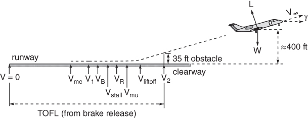
Figure 14.1 Sizing for takeoff.
For sizing, field length calculations are at the sea level standard day (no wind) and at a zero airfield gradient of paved runway. For further simplification, drag changes are ignored during the transition phase of lift‐off to clear the obstacle (flaring takes about two to four seconds); in words, the equations applied to Vlift‐off are extended to V2.
Chapter 15 addresses takeoff performance in detail. Eq. (15.8) gives

where dV/dt = a is the instantaneous acceleration and V is the instantaneous velocity. The aircraft on the ground encounters rolling friction (coefficient μ = 0.025 for a paved, metalled runway). Average acceleration, ā, is taken at 0.7V2. FAR requires V2 = 1.2Vstall. This gives V2 2 = [2 × 1.44 × (W/SW)]/(ρCLstall). An aircraft stalls at CLmax. By substituting the value of V2, the Eq. 14.1 reduces to:
Its simplified expression for all engines operating is:
Writing in terms of wing loading Eq. 14.2 can be written as
where average acceleration, ā = F/m and applied force F = (T − D) − μ(W − L).
Note that, until lift‐off is achieved, W > L and F is the average value at 0.7V2.
Substituting in Eq. 14.3 it becomes
In the foot–pound system (FPS) it can be written as (ρ = 0.00238 slugs and g = 32.2 ft s−2)
In the SI system it becomes (ρ = 1.225 kg m−3 and g = 9.81 m s−2)
here W/SW is in N m−2 to remain in alignment with the units of thrust in newtons.
Checking of the second‐segment climb gradient occurs after aircraft drag estimation, which is explained in Chapter 11. If climb gradient falls short of the requirement, then the TSLS must be increased. In general, the stringent TOFL requirements also likely to satisfy the second segment climb gradient.
14.3.1.1 Civil Aircraft Design: Takeoff
The contribution of the last three terms (−D/T − μW/T + μL/T) in Eq. 14.4 is minimal and can be omitted at this stage for the sizing calculation. In addition, for the one‐engine‐inoperative condition after the decision speed V1, the acceleration slows down, making the TOFL longer than the all engines operative case. Therefore, in the sizing computations to produce the specified TOFL, further simplification is possible by applying a semi‐empirical correction factor primarily to compensate for loss of an engine. The correction factors are as follows [2]; all sizing calculations are performed at the MTOW and with TSLS.
For two engines, use a factor of 0.5 (loss of thrust by a half).
Then, Eqs. (14.6a) and (14.6b) in the FPS system reduces to:
For the SI system:
For three engines, use a factor of 0.66 (loss of thrust by a third). Then, Eq. (14.6) in the FPS system reduces to:
For the SI system:
For four engines, use a factor of 0.75 (loss of thrust by a quarter). Then, Eq. (14.6) in the FPS system reduces to:
For the SI system:
14.3.1.2 Military Aircraft Design: Takeoff
Because military aircraft mostly have a single engine, there is no requirement for one engine being inoperative; ejection is the best solution if the aircraft cannot be landed safely. Therefore, Eqs. (14.6a) and (14.6b) can be directly applied (for a multiengine design, the one‐engine‐inoperative case, generally, uses measures similar to the civil aircraft case). In the FPS system, this can be written as:
In the SI system, it becomes:
Military aircraft have a thrust, TSLS/W, that is substantially higher than civil aircraft, which makes (D/T − μW/T + μL/T) even smaller. Therefore, for a single‐engine aircraft, no correction is needed and the simplified equations are as follows:
In the FPS system, this can be written as:
In the SI system, this becomes:
14.3.2 Sizing for the Initial Rate of Climb (All Engines Operating)
The initial unaccelerated rate of climb is a user specification and not a FAR requirement; this is when the aircraft is heaviest in climb. In general, the FAR requirement for the one‐engine‐inoperative gradient provides sufficient margin to give a satisfactory all‐engine initial climb rate. However, from the operational perspective, higher rates of climb are in demand when it is sized accordingly. Military aircraft (some with a single engine) requirements stipulate faster climb rates and sizing for the initial climb rate is important. The methodology for aircraft sized to the initial climb rate is described in this section. Sizing exercise for climb is at unaccelerated rate of climb. Figure 14.2 shows a typical climb trajectory.

Figure 14.2 Aircraft climb trajectory.
For a steady‐state climb, the Eq. (15.5) gives the expression for rate of climb, RC = V × sin γ.
Steady‐state force equilibrium gives T = D + W × sin γ or sin γ = (T − D)/W.
This gives
Equation 14.12 is written as
Equation 14.13 is based on climb thrust rating, which is lower than TSLS. Equation 14.13 needs to be written in terms of TSLS. The ratio, TSLS/T = kcl varies depending on the engine bypass ratio (BPR).
The drag polar is now required to compute the relationships given in Equation 14.14.
14.3.3 Sizing to Meet Initial Cruise
There are no FAR or Milspec regulations to meet the initial cruise speed; initial cruise capability is a user requirement. Therefore, both civil and military aircraft sizing for initial cruise use the same equations. At a steady‐state level flight, thrust required (aeroplane drag, D) = thrust available (Ta); that is:
Dividing both sides of the equation by the initial cruise weight, Win_cr = k × MTOW due to fuel burned to climb to the initial cruise altitude. The factor k lies between 0.95 and 0.98 (climb performance details are not available during the conceptual design phase), depending on the operating altitude for the class of aircraft, and it can be fine‐tuned through iterations: in the coursework exercise, one round of iterations is sufficient. The factor cancels out in the following equation but is required later. Henceforth, in this part of cruise sizing, W represents the MTOW, in line with the takeoff sizing:
The drag polar gives the CD value to correspond to the initial cruise CL (because they are non‐dimensional, both the FPS and SI systems provide the same values). Initial cruise:
The thrust‐to‐weight ratio sizing for initial cruise capability is expressed in terms of TSLS. Eq. 14.18 is based on the maximum cruise thrust rating, which is lower than the TSLS. Eq. 14.18 must be written in terms of TSLS. The ratio, TSLS/Ta = kcr; varies depending on the engine BPR. The factor kcr is computed from the engine data supplied. Then, Eq. 14.18 can be rewritten as:
Variation in wing size affects aircraft weight and drag. The question now is: How does the CD change with changes in W and SW? (Ta changes do not affect the drag because it is assumed that the physical size of an engine is not affected by small changes in thrust.) The solution method is to work with the wing only – first by scaling the wing for each case and then by estimating the changes in weight and drag and iterating – which is an involved process.
This book simplifies the method by using the same drag polar for all wing‐loadings (W/SW) with little loss of accuracy. As the wing size is scaled up or down (the AR invariant), it changes the parasite drag. The induced drag changes as the aircraft weight increases or decreases. However, the CD increase with wing growth is divided by a larger wing, which keeps the CD change minimal.
14.3.4 Sizing for Landing Distance
The most critical case is when an aircraft must land at its maximum landing weight of 0.98 MTOW. In an emergency, an aircraft lands at the same airport for an aborted takeoff procedure, assuming a 2% weight loss due to fuel burn in order to make the return circuit. Pilots prefer to approach as slow as possible for ease of handling at landing.
For the Bizjet class of aircraft, the approach velocity, Vapp (FAR requirement at 1.3 Vstall) is less than 125 kts to ensure that it is not constrained by the minimum control speed, Vc. Wing CLstall is at the landing flap and slat setting. For sizing purposes, an engine is set to the idle rating to produce zero thrust.
At landing Vapp = 1.3 Vstall.
Therefore,
14.4 Coursework Exercise – Civil Aircraft Design (Bizjet)
Both the FPS and the SI units are used for the worked‐out examples. Sizing calculations require the engine data in order to obtain the k factors used. The Bizjet drag polar is provided in Figure 11.2.
14.4.1 Takeoff
Requirements. TOFL 4400 ft (1341 m) to clear a 35‐ft height at ISA + sea level. The maximum lift coefficient at takeoff (i.e. flaps down to 20° and no slat) is CLstall(TO) = 1.9 (obtained from testing and computational fluid dynamics (CFD) analysis). Installation losses are taken to 7% that reduces takeoff thrust to 0.93 TSLS. Using Eq. (14.7a), the expression reduces to:
Using Eq. (14.7a), the expression reduces to W/SW = 4400 × 1.9 × (0.93 × TSLS/W)/37.5 = 207.3 × (T/W).
Using Eq. (14.7b), it becomes W/SW = 4.173 × 1341 × 1.9 × (0.93 × TSLS/W) = 9889.2 × (TSLS/W)
The result is computed in Table 14.1.
Table 14.1 Bizjet takeoff sizing calculations.
| W/SW (FPS – lb ft−2) | 40 | 50 | 60 | 70 | 80 |
| W/SW (SI – N m−2) | 1916.9 | 2395.6 | 2874.3 | 3353.7 | 3832.77 |
| TSLS/W (installed) | 0.193 | 0.24 | 0.29 | 0.338 | 0.386 |
The industry must also examine other takeoff requirements (e.g. an unprepared runway) and hot and high ambient conditions.
14.4.2 Initial Climb
From the market requirements, an initial climb starts at an 1400‐ft altitude (ρ = 0.00232 slugs/ft3) at a speed VEAS = 250 kt (Mach 0.38) = 250 × 1.68781 = 422 ft s−1 (128.6 m s−1) and the required rate of climb, RC = 2600 ft min−1 (792.5 m min−1) = 43.33 ft s−1 (13.2 m s−1). For the class of TFE731 engine data, Figure 13.3 gives the uninstalled kcl = T/TSLS = 0.705. Taking 5% installation loss during climb, the installed kcl = T/TSLS = 0.95 × 0.705 = 0.67 that gives TSLS/T = 1.5. The undercarriage and high‐lift devices are in a retracted position. The result is computed in Table 14.2.
Table 14.2 Bizjet climb sizing calculations (use Figure 11.2 for the drag polar).
| W/SW (lb ft−2) | 40 | 50 | 60 | 70 | 80 |
| W/SW (N m−2) | 1916.9 | 2395.6 | 2874.3 | 3353.7 | 3832.77 |
| CLclimb | 0.194 | 0.242 | 0.290 | 0.339 | 0.378 |
| CD (from drag polar) | 0.024 | 0.0246 | 0.0256 | 0.0266 | 0.0282 |
| TSLS/W (installed) | 0.34 | 0.31 | 0.286 | 0.272 | 0.265 |
Lift coefficient,
Using Eq. 14.14,
14.4.3 Cruise
Requirements. Initial cruise speed must meet the high‐speed cruise (HSC) at Mach 0.75 and at 41 000 ft (flying higher than bigger jets in less congested traffic corridors). Using Eq. 14.19, the result is computed in Table 14.3 (for the initial cruise aircraft weight use k = 0.972 in.).
Table 14.3 Bizjet cruise sizing.
| W/SW (lb ft−2) | 40 | 50 | 60 | 70 | 80 | |
| W/SW (N m−2) | 1916.9 | 2395.6 | 2874.3 | 3353.7 | 3832.77 | |
| CL | 0.271 | 0.339 | 0.4064 | 0.474 | 0.542 | 0.619 |
| CD (from drag polar) | 0.0255 | 0.0269 | 0.0295 | 0.033 | 0.0368 | |
| T/W @ 41 000 ft | 0.36 | 0.305 | 0.278 | 0.267 | 0.26 |
In FPS at 41 000 ft:
In SI at 12 519 m altitude:
Equation 14.18 gives the initial cruise:
Equation 14.19 gives:
For the class of TFE731 engine data, Figure 13.4 gives the uninstalled kcr = T/TSLS = 0.23. Taking 4% installation loss during cruise, the installed kcl = T/TSLS = 0.94 × 0.23 = 0.222 that gives TSLS/T = 4.5.
In FPS:
In SI:
Using Figure 11.2 for the drag polar, Table 14.3 gives the computed values for Bizjet cruise sizing.
14.4.4 Landing
From the market requirements, Vapp = 120 knots = 120 × 1.68781 = 202.5 ft s−1 (61.72 m s−1). Landing CLmax = 2.1 at a 40° flap setting (from testing and CFD analysis). For sizing purposes, the engine is set to the idle rating, producing zero thrust. Using Eq. 14.22 the following is obtained.
In the FPS system, W/SW = 0.311 × 0.002378 × 2.1 × (202.5)2 = 63.8 lb ft−2. In the SI system, W/SW = 0.311 × 1.225 × 2.1 × (61.72)2 = 3052 N m−2. Because the thrust is zero (i.e. idle rating) at landing, the W/SW remains constant.
14.5 Sizing Analysis – Civil Aircraft (Bizjet)
The four sizing relationships for wing loading, W/SW, and thrust loading, TSLS/W, meet (i) takeoff, (ii) approach speed for landing, (iii) initial cruise speed and (iv) initial climb rate. These are plotted in Figure 14.3. The circled point in Figure 14.3 is the most suitable for satisfying all four requirements simultaneously. To ensure performance, there is a tendency to use a slightly higher thrust loading TSLS/W; in this case, the choice becomes as follows.
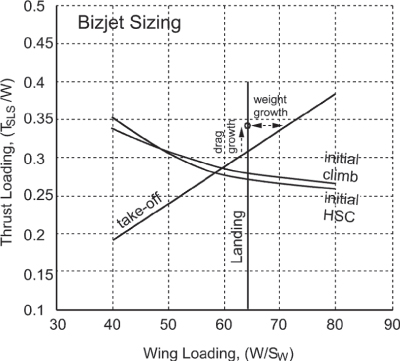
Figure 14.3 Aircraft sizing – civil aircraft.
TSLS/W = 0.34 at a wing loading of W/SW = 64 lb ft−2 (2894 N m−2). This keeps some margin for future weight growth through modifications and some drag growth as shown in Figure 14.3.
So far, the Bizjet aircraft data has been given. This chapter uses the Bizjet size measurements to check the extent of differences in aircraft geometry, engine size and weight. Now is the time for the iterations required to fine‐tune the given preliminary configuration. At 20 720 lb (9400 kg) MTOM, the wing planform area is 325 ft2, close to the original area of 323 ft2; hence, no iteration is required. Otherwise, it is necessary to revisit the empennage sizing and revise the weight estimates. The TSLS per engine then becomes 0.34 × 20 720/2 = 3523 lbs ≈ 3500 lb/engine. This is very close to the TFE731‐20 class of engine; therefore, the engine size and weight remain the same. For this reason, iteration is avoided; otherwise, it must be carried out to fine‐tune the mass estimation.
The entire sizing exercise could have been conducted well in advance, even before a configuration was settled – if the chief designer's past experience could guesstimate a close drag polar and MTOM. Statistical data of past designs are useful in guesstimating aircraft close to an existing design. Generating a drag polar requires some experience with extraction from statistical data. Subsequently, the sizing exercise is fine‐tuned to better accuracy.
In the industry, more considerations are addressed at this stage – for example, what type of variant design in the basic size can satisfy at least one larger and one smaller capacity (i.e. payload) size. Each design may have to be further varied for more refined variant designs.
14.5.1 Variants in the Family of Aircraft Designs
The family concept of aircraft design is discussed in previous chapters and highlighted again at the beginning of this chapter. Maintaining large component commonality (genes) in a family is a definite way to reduce design and manufacturing costs – in other words, ‘design one and get two or more almost free’. This encompasses a much larger market area and, hence, increased sales to generate resources for the manufacturer and nation. The amortisation is distributed over larger numbers, thereby reducing aircraft costs.
Today, all manufacturers produce a family of derivative variants. The Airbus320 series has four variants and more than 3000 have been sold. The Boeing737 family has six variants, offered for nearly four decades, and nearly 6000 have been sold. It is obvious that in three decades, aircraft manufacturers have continuously updated later designs with newer technologies. The latest version of the Boeing737–900 has vastly improved technology compared to the late 1960s 737–100 model. The latest design has a different wing; the resources generated by large sales volumes encourage investing in upgrades – in this case, a significant investment was made in a new wing, advanced cockpit/systems, and better avionics, which has resulted in continuing strong sales in a fiercely competitive market.
The variant concept is market and role driven, keeping pace with technology advancements. Of course, derivatives in the family are not the optimum size (more so in civil aircraft design), but they are a satisfactory size that meets the demands. The unit‐cost reduction, as a result of component commonalities, must compromise with the non‐optimum situation of a slight increase in fuel burn. Readers are referred to Figure 16.6, which highlights the aircraft unit‐cost contribution to DOC as more than three to four times the cost of fuel, depending on payload‐range capability. The worked‐out examples in the next section offer an idea of three variants in the family of aircraft.
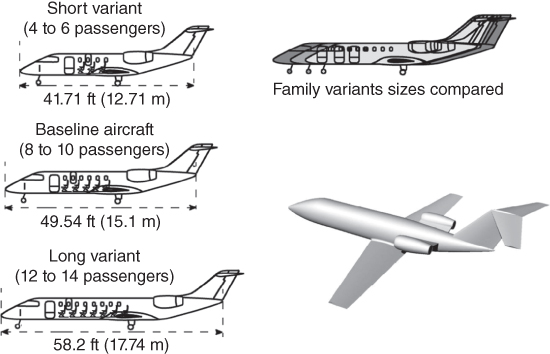
Figure 14.4 Variant designs in the family of civil aircraft.
14.5.2 Bizjet Family
Figure 14.4 shows the final configuration of the family of ; the baseline aircraft is in the middle. It proposes one smaller (i.e. 4–6 passengers) and one larger (i.e. 14–16 passengers) variant from the baseline design that carries 10–12 passengers by subtracting and adding fuselage plugs from the front and aft of the wing box. The baseline and variant details are worked out in Section 8.9. Table 14.4 gives the summary of the Bizjet variants.
Table 14.4 Bizjet family variant summary SW = 323 ft2.
| Short variant | Baseline | Long variant | |
| MTOM kg (lb) | 7800 (17190) | 9400 (20720) | 10 900 (23580) |
| W/SW (lb ft−2) | 53.22 | 64.0 | 73.0a |
| TSLS/W | (0.33) | 0.34 | (0.35) |
| TSLS/per engine‐lb | 2836 | 3560 | 4130 |
aLong variant requires superior high‐lift device for landing.
The short variant engine is derated by about 17% resulting in slightly lower engine weight and the long variant engine is up‐rated by about 15% resulting in slightly higher engine weight.
14.6 Coursework Exercise – Military Aircraft (AJT)
Military designs follow Milspecs and not FAR for airworthiness requirements. Both FPS and SI units are worked out in the examples. Figure 11.17 gives the AJT drag polar. The military aircraft example of AJT operates in two takeoff weights as (i) at normal training configuration (NTC – clean) at 4800 kg and (ii) at fully loaded for armament training at 6800 kg, that is, a growth of 41.7%. In this example the NTC is more critical to meet the specification of TOFL = 800 m). The readers may work out both the cases. The fully loaded aircraft needs to satisfy the longer field length requirement of 1800 m (<6000 ft), the rest, for example, climb and cruise capabilities, are taken as fallout of the design. After the armament practice run the payload is dropped and the landing weight is the same for both the missions. It may be noted that the AJT should have a close air support (CAS) version. Only initial MTOW and wing area are required for sizing.
14.6.1 Takeoff – Military Aircraft
Requirements. TOFL = 800 m (≈2600 ft) to clear 35 ft (10.7 m) at ISA + sea at NTC. The maximum lift coefficient at TO (20° flaps down and no slat) is taken as CLmax_TO = CLstall_TO = 1.85. Installation is taken at 3.5%.
Using Eq. (14.11a), the expression becomes (in FPS system)
Using Eq. (14.11b), it becomes (in SI system)
The result is computed in Table 14.5 and listed in tabular form.
Table 14.5 AJT takeoff sizing.
| W/SW (FPS – lb ft−2) | 40 | 50 | 60 | 70 | 80 | 90 |
| W/SW (SI – N m−2) | 1916.2 | 2395.6 | 2874.3 | 3353.7 | 3832.77 | 4311.5 |
| TSLS/W (uninstalled) | 0.163 | 0.207 | 0.244 | 0.284 | 0.324 | 0.366 |
14.6.2 Initial Climb – Military Aircraft
From market requirement, initial climb speed V = 350 kt = 350 × 1.68781 = 590.7 ft s−1 and the required rate of climb, RC = 10 000 ft min−1 (50 m s−1) = 164 ft s−1 (50 m s−1). From the Adour 861 class engine data TSLS/T ratio, kcl = 1.06. The result is computed in Table 14.6.
Table 14.6 AJT climb sizing calculations.
| W/S (lb ft−2) | 40 | 50 | 60 | 70 | 80 |
| W/S (N m−2) | 1916.2 | 2395.6 | 2874.3 | 3353.7 | 3832.77 |
| CLclimb | 0.097 | 0.12 | 0.145 | 0.169 | 0.193 |
| CD (from Figure 14.16) | 0.0222 | 0.0225 | 0.0258 | 0.026 | 0.0263 |
| TSLS/W (uninstalled) | 0.538 | 0.492 | 0.483 | 0.457 | 0.439 |
Lift coefficient,
Using Eq. 14.15,
14.6.3 Cruise – Military Aircraft
Market Specification. Initial cruise speed and altitude is 0.75 Mach and 36 000 ft (most of training is takes place below the tropopause), for the initial cruise aircraft weight take, k = 0.975 in Eq. 14.14. The result is computed in Table 14.7.
In FPS
In SI,
Equation 14.18 gives initial cruise
Equation 14.19 gives.
In FPS
In SI
Once again, make a table (see Table 14.7) and draw a plot.
Table 14.7 AJT cruise sizing.
| W/SW (lb ft−2) | 50 | 60 | 70 | 80 | 100 |
| W/SW (N m−2) | 2395.6 | 2874.3 | 3353.7 | 3832.8 | 4791 |
| CL | 0.262 | 0.314 | 0.367 | 0.419 | 0.524 |
| CD | 0.026 | 0.0292 | 0.0315 | 0.035 | 0.042 |
| TSLS/W @ 41 000 ft | 0.346 | 0.324 | 0.30 | 0.29 | 0.279 |
14.6.4 Landing – Military Aircraft
From the market requirements,
Landing CLstall = 2.5 at a 40° double slotted flap setting.
Using Eq. 14.22,
In FPS system,
In the SI system,
Because at landing the thrust is taken to be zero, the W/SW remains constant.
14.6.5 Sizing for the Turn Requirement of 4g at Sea Level
In a way, turn sizing is relatively simple and here the parabolic drag polar AJT is used to make use of the equation derived in Chapter 15. The approximated AJT parabolic drag polar is given in Section 11.20.1 as follows.
The turn requirement is n = 4 at sea level (STD) day, but is stipulation for speed at which it can be achieved. It gives the opportunity to initiate sizing analyses in many ways different from these methods. The turn sizing is carried out by establishing the relationship between, wing loading, W/SW, and thrust loading TSLS/W at n = 4, the turn speed that has to be establish. Use Eq. (15.58) (derived in the next chapter) and evaluate at three speeds at Mach 0.5 (V = 558.25 ft s−1), Mach 0.55 (V = 614.075 ft s−1) and Mach 0.6 (V = 669.9 ft s−1).
 , on substituting the numeric values, the following is obtained.

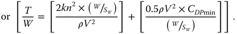
On substituting the numerical values of ρ = 0.002378 slugs/ft3, k = 0.07 and CDPmin = 0.0212.
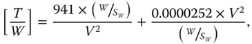
where T is the installed thrust at maximum continuous rating.
Aircraft sizing thrust loading is expressed in terms of uninstalled sea level static thrust at maximum takeoff rating, TSLS_unins. Maximum continuous rating is taken at 90% of maximum takeoff rating and installation loss is taken as 3.5%. That makes:
installed thrust at maximum continuous rating,
Tables 14.8–14.10 show the (T/W) values at three (W/SW) cases of 50 lb ft−2, 60 lb ft−2 and 70 lb ft−2 for the three speeds at Mach 0.5, 0.55 and 0.6.
Table 14.8 Mach 0.5 (V = 558.25 ft s−1), V2 = 311 587.2 (ft s−1)2.
| W/SW (lb ft−2) | 50 | 60 | 70 |
| V2 | 311 587.2 | 311 587.2 | 311 587.2 |
| 0.151 001 | 0.181 201 | 0.211 401 5 | |
| 0.155 794 | 0.129 828 | 0.111 281 1 | |
| T/W | 0.306 795 | 0.311 029 | 0.322 682 6 |
| TSLS/W | 0.352 814 | 0.357 684 | 0.371 085 |
Table 14.9 Mach 0.55 (V = 614.075 ft s−1), V2 = 376 996 (ft s−1)2.
| W/SW (lb ft−2) | 50 | 60 | 70 |
| 0.124 802 | 0.149 763 | 0.174 723 3 | |
| 0.190 006 | 0.157 082 | 0.135 718 6 | |
| T/W | 0.314 808 | 0.306 845 | 0.310 441 9 |
| TSLS/W | 0.362 03 | 0.352 871 | 0.3570 082 |
Table 14.10 Mach 0.6 (V = 669.9 ft s−1), V2 = 448 632 (ft s−1)2.
| W/SW (lb ft−2) | 50 | 60 | 70 |
| 0.104 874 | 0.125 849 | 0.146 824 1 | |
| 0.226 111 | 0.188 425 | 0.161 507 5 | |
| T/W | 0.330 985 | 0.314 275 | 0.308 331 6 |
| TSLS/W | 0.380 633 | 0.361 416 | 0.354 581 4 |
Tables 14.8–14.10 give three lines with close values (T/W). Only the line for Mach 0.55 is plotted in Figure 14.5 as the middle one of the three. With the excess thrust available, AJT can turn at a higher n (see Chapter 15).
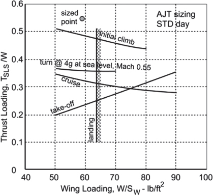
Figure 14.5 Aircraft sizing – AJT (military).
14.7 Sizing Analysis – Military Aircraft (AJT)
The methodology for military aircraft is the same as in the case of civil aircraft sizing and engine matching. The five sizing relationships between wing loading, W/SW, and thrust loading, TSLS/W, would meet (i) takeoff, (ii) approach speed for landing, (iii) initial cruise speed, (iv) initial climb rate and (v) turn rate capability. These are plotted in Figure 14.5.
Military aircraft sizing poses an interesting situation. The variant in combat role, for example, in a CAS role has to carry more armament load externally contributing to drag rise. The overall geometry does not change much except the front fuselage is now redesigned for one pilot saving a weight of about 100 kg (the weight of seat, escape system etc. are replaced by radar, combat avionics). The aircraft still has the same engine tweaked to up‐rated thrust level.
Therefore, a conservative sizing of AJT should benefit CAS growth. Figure 14.5 shows the sizing point is at slightly lower wing loading at W/SW = 59 lb ft−2 to benefit CAS performance. Thrust loading is taken as TSLS/W = 0.55. The circled point in Figure 14.5 satisfies all requirements simultaneously. If required, iteration can be carried out with a slightly higher value of TSLS/W to meet nmax = 7 (see Section 15.11.8) as well as benefit the takeoff and initial climb performance of AJT with full practise armament load.
Chapter 10 worked out the mass of the preliminary of AJT aircraft as:
MTOM = 4800 kg (10 582 lb) at NTC, which gives the matched engine thrust TSLS = 0.55 × 10,582 ≈ 5,830 lb (25,933 N).
Checking out with the sized wing loading W/SW = 59 lb ft−2, the wing area comes out at 185 ft2 (17.2 m2) about 1% error from the preliminary wing area, hence it remains unchanged. The matched engine thrust gives a lower value compared to the statistical estimate of 5860 lb, which is good. Once again, iteration is avoided.
14.7.1 Single Seat Variants in the Family of Aircraft Designs
Military aircraft are no exceptions in offering variant designs depending on their mission role, in addition to the typical ‘payload‐range’ variation. The F16 and F18 have had modifications since they first appeared with an increasing envelope of combat capabilities. The F18 has increased in size. The BAE Hawk100 jet trainer has produced a single seat close support combat derivative, the Hawk200.
The CAS role aircraft is the only variant of the AJT aircraft (Figure 14.6). The details on how it is achieved with associated design changes are described next.
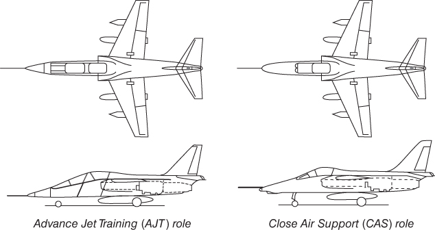
Figure 14.6 Variant designs in the family of military aircraft.
14.7.1.1 Configuration
Configuration of CAS aircraft variant is achieved by splitting the AJT front fuselage, then replacing the tandem seat arrangement with a single seat cockpit. The length could be kept the same as the nose cone needs to house more powerful acquisition radar. The front loading of radar and single pilot is placed in such a way that the CG location is kept undisturbed. Wing area = 17 m2 (183 ft2). The bold values presented highlight the important parameters.
| Weights | AJT | CAS |
| Clean aircraft MTOM | 4800 (10 582 lb) | 5000 (11 023 lb) |
| Wing loadinga, W/SW | 282 kg/m2 (57.8 lb ft−2) | 294 kg/m2 (60.23 lb/ft2). |
| MTOM kg (lb) | 6500 (14 326 lb) | 7400 (16 310 lb) |
| Wing area, SW | 17 m (183 ft2) | 17 m (183 ft2) |
| Wing loading, W/SW | 382.5 kg m−2 (78.3 lb ft−2) | 435.3 kg m−2 (89.1 lb ft−2). |
Sized wing loading for AJT at NTC came out close to it.
Armament and fuel could be traded for range. Drop tanks could be used for ferry range.
14.7.1.2 Thrust
The CAS variant would require a 30% higher engine thrust variant. This is possible without any change in external dimension but would incur an increase of 60 kg in engine mass.
CAS turbofan (has small bypass) thrust = 1.3 × 5300 ≈ 6900 lb (30 700 N).
Thrust loading at MTOM becomes: TSLS/W = 0.417 (a satisfactory value).
14.7.1.3 Drag
The drag level of the clean AJT and CAS aircraft may be considered to be about the same. There would be an increase of drag on account of the weapon load. For the CAS aircraft, there is a wide variety, but to give a general perception, the typical drag coefficient increment for armament load is CDπ = 0.25 (includes interference effect) each for five hard points as weapon carrier. Weapon drag is based on maximum cross section (say 0.8 ft2) area of the weapons.
Parasite drag increment, ΔCDpmin = (5 × 0.25 × 0.8)/183 = 0.0055, where SW = 183 ft2.
14.8 Aircraft Sizing Studies and Sensitivity Analyses
Aircraft sizing studies and sensitivity analyses are not exactly the same thing as outlined next. Together with both sizing and sensitivity study exercises, the aircraft designers are able to find an optimised or satisfying design to satisfy the certification agency and customer simultaneously. The designers and the users will have better insights to make better choices.
14.8.1 Civil Aircraft Sizing Studies
Aircraft sizing exercise freezes aircraft to a unique geometry with little scope to make variation as shown in Figure 14.3 for the Bizjet. In these kinds of studies, aircraft performance requirements from the Federal Aviation Administration (FAA) and specification (customer) are given as: (i) takeoff field length and climb gradients, (ii) initial en‐route climb, (iii) initial HSC capability and (iv) LFL and climb gradients at baulked landing are simultaneously satisfied with a matched engine and a unique solution emerges. To search for a compromising to offer a family of variants it depends on objectives, for example, the degree of component components can be retained.
It is a broad‐based analysis and could be extensive. Basically, it is an optimisation process to find the best value providing opportunities to make any compromise, if required. The easiest method is to take one variable at a time in a parametric search to find on how it is affecting other parameters. Normally, the variations are made in small steps to keep changes in the affecting parameters within the ranges of acceptable errors. In civil aircraft design, the study should continue to examining the objective function, say the DOC. Typically, the results are shown in carpet plots (Figure 14.7) studying up to as many as five variables [5]. This carpet plot shows four variables in one graph with mutual inter‐dependency. It shows how aircraft DOC is affected with aircraft drag change, fuel price and aircraft cost for an Airbus 320 class aircraft.

Figure 14.7 Typical parametric study of a mid‐sized aircraft (A320 class) (shown in a carpet plot showing DOC variations with aircraft drag and costs).
Apart from parametric method of searching there are theoretical methods available. The simpler ones are the Simplex and Gradient methods; those are used in the industry, but the parametric method is most popular.
14.8.1.1 Military Aircraft Sizing Studies
Aircraft sizing exercise freezes aircraft to a unique geometry with little scope to make variations as shown in Figure 14.3 for the Bizjet. The aircraft sizing exercise freezes aircraft to a unique geometry with little scope for variation as shown in Figure 14.5 for the AJT.
In aircraft design sensitivity can be made on determining individual component geometries, for example, for wing examine how its area, AR, thickness to chord ratio, sweep and so on, affects aircraft capabilities as shown in Table 14.11 for the AJT. An example of AJT wing geometry sensitivity study is given next involving what happens with small changes in wing reference area, SW, aspect ratio, AR, aerofoil thickness to chord ratio, t/c, and wing quarter chord sweep, Λ¼.
Table 14.11 AJT sensitivity study.
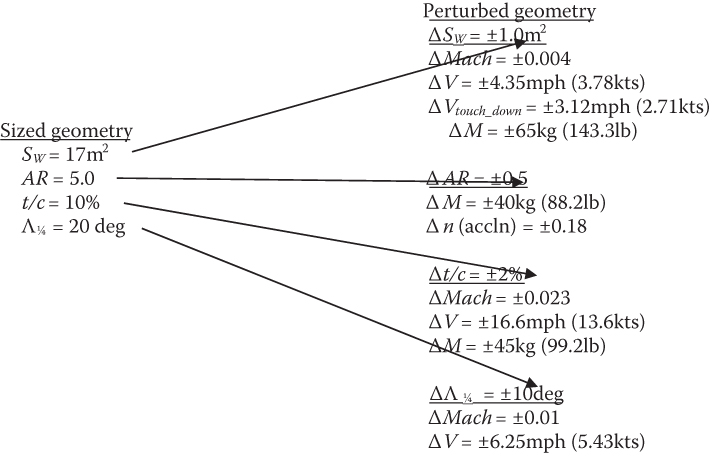 |
A more refined analysis could be made with a detailed sensitivity study on various design parameters, such as other geometrical details, materials, structural layout and so on, to address cost versus performance issues to arrive at a ‘satisfying’ design. This may require some local optimisation with full awareness that the global optimisation is not sacrificed. While a broad‐based MDO is the ultimate goal, dealing with large number of parameters in a sophisticated algorithm may not prove easy. It is still researched intensively within academic circles, but industry tends to use MDO in a conservative manner if required in a parametric search, tackling one variable at a time. Industry cannot afford to take risks with any unproven algorithm just because it is elegant bearing promise. Industry takes a more holistic approach to minimise costs without sacrificing safety but may compromise on performance if it pays.
14.9 Discussion
Aircraft sizing exercise can keep open the possibilities for aircraft future growth potential. If possible, even a radically new design can salvage components from older design to maintain parts commonalities.
This culminating section presents some discussion on the classroom examples and their performances options are presented. The sizing exercise gives the simultaneous solution to satisfy the airworthiness and the market requirements. This is an activity in the conceptual design phase when few details about aircraft data are available. The sizing exercise requires specific aircraft performance evaluation in a concise manner using the relevant equations derived thus far. Sizing studies are management issues those are reviewed along with the potential customers to decide to give the go‐ahead or not. In sizing and engine matching exercise, the wing loading (W/SW) and thrust loading (T/W) are the dictating parameters appear in equations for takeoff, second segment climb, en‐route climb and maximum speed capability. The first two are FAR requirements and the last two are customer requirements. Information on detailed engine performance is not required during the sizing exercise; projected rubberised engine data are used during the sizing and engine matching studies. Payload‐range capability of the proposed design needs to be demonstrated as the customer requires. Subsequently, with the details of engine performance and aircraft data, relevant aircraft performance analyses are carried out more accurately to satisfy airworthiness and market requirements.
Once the go‐ahead is obtained, then a full blown detailed definition study ensues as Phase II activities with large financial commitments. Refinement continues until accurate data are obtained from flight tests and other refined analyses. Most of the most important aircraft performance equations are in this book in reasonable details supported by worked‐out examples.
Sizing in Figure 14.3 (Bizjet) shows the lines of constraints for the various requirements. The sizing point to satisfy all requirements would show different level of margins for each capability. Typically, initial en‐route climb rate is the most critical to sizing. Therefore, the takeoff and maximum speed capabilities have considerable margin, which is good as the aircraft can do better than what is required.
From the statistics, experience shows that aircraft mass grows with time. This occurs primarily on account of modifications arising out of mostly from minor design changes and with changing requirements, sometimes even before the first delivery is made. If the new requirements demand a large number of changes then civil aircraft design may appear as a new variant but military aircraft hold on a little longer before a new variant emerges. It is therefore prudent for the designers to keep some margin, especially with some reserve thrust capability, that is, keep the thrust loading, (T/W), slightly higher to begin with. Re‐engineering with an up‐rated version is expensive.
It can be seen that field performance would require a bigger wing planform area (SW) than at cruise. It is advisable to keep wing area as small as possible (i.e. high wing loading) by incorporating a superior high‐lift capability, which is not only heavy but also expensive. Designers must seek compromise to minimise operating costs. No iteration was needed for the designs worked out in the book.
Section 15.3 derived all the necessary relations to estimate the aircraft cruise segment required to compute aircraft mission payload‐range capability and the block time and block fuel required for the mission. In summary, both the close form analytical method for various options for trend analyses using parabolic drag polar and numerical analyses using actual drag polar are analysed and the results are compared. The question now is which method is to be applied when as each one has its own reason of application.
The first thing that needs to be pointed out that actual drag polar is more accurate as it is obtained through proven semi‐empirical methods and refined by tests (wind‐tunnel and flight). Operators require an accurate manual to maximise city‐pair mission planning. To establish the best possibility, for example, to decide the speed and altitude for the sector, is not easy. Here, close form analysis assists to quickly provide answers for the best possibilities. This is then fine‐tuned trough flight tests and then incorporated in the operator's manual; nowadays it is digitised and stored at several places, on ground and in the aircraft. In the past flight engineers had to compute prior to any sortie and keep monitored during the sortie flight. By today's standard it is a laborious and time consuming process as today these can be obtained almost instantaneously by the press of buttons.
The sizing point in Figure 14.3 gives a wing loading, W/SW = 64 lb ft−2 and a thrust loading, T/W = 0.34. It may be noted that there is little margin given for the landing requirement. The maximum landing mass for this design is at 95% of MTOM. A margin for 10% weight growth corresponding drag growth is accommodated in the sizing exercise. Commonality of undercarriage for all variants would start with the design for the heaviest, that is, the growth variant and its bulky components are shaved to lighten them for lower weights. The middle variant is taken as the baseline version. Its undercarriage can be made to accept MTOM growth as a result of OEW (Operating Empty Weight) growth instead of making the wing larger.
It should be borne in mind the recommendation is that civil aircraft should come in a family of variants to cover wider market demand to maximise sale. Truly speaking, none of the three variants are optimised although the baseline is carefully sized in the middle to accept one larger and one smaller variant. Even when the development cost is front loaded, the cost of development of the variant aircraft is low by sharing the component commonality. The low cost is then translated to lowering aircraft price, which can absorb the operating costs of the slightly non‐optimised designs.
It is interesting to examine the design philosophy of the Boeing737 family and the Airbus320 family of aircraft variants in the same market arena. Together more than 8000 aircraft have been sold in the world market. This is a no small achievement in engineering. The cost of these aircraft is about $50 million apiece (2005). For airlines with deregulated fare structures, making a profit involves a complex dynamics of design and operation. The cost and operational scenario changes from time to time, for example, rise of fuel cost, terrorist threats and so on.
As early as the 1960s, Boeing saw the potential of keeping component commonality in offering new designs. The B707 was one of the earliest commercial jet transport aircraft carrying passengers. It was followed by a shorter version B720. Strictly speaking the B707 fuselage relied on the KC135 tanker design of the 1950s. From the four‐engine B707 came the three‐engine B727 and then the two‐engine B737, both retaining considerable fuselage commonality. This was one the earliest attempts to utilise the benefits of maintaining component commonality. Subsequently, the B737 started to emerge in different sizes of variants maximising component commonality. The original B737‐100 was the baseline design and all other variants that came later, up to the B737‐900. It posed certain constraints, especially on the undercarriage length. On the other hand, the A320 serving as the baseline design was in the middle of the family, its growth variant is the A321 and shrunk variants are the A319 and A318. Figure 7.3 gives a good study on how the OEW is affected by the two examples of family of variants. A baseline aircraft starting at the middle of the family would be better optimised and hence in principle would offer a better opportunity to lower production cost of the variants in the family.
Simultaneous failure of two engines of a four‐engine aircraft is extremely rare. If it happens after the decision speed and if there is not enough clearway available then it will catastrophic. If the climb gradient is not in conflict with the terrain of operation then it is better to takeoff with higher flap settings. If a longer runway is available then lower flap setting could be used. Takeoff speed schedules can slightly exceed the FAR requirements that stipulate the minimum values. There have been cases of all engine failures occurring at cruise on account of volcanic ash in the atmosphere (also in the rare event of fuel starvation). Fortunately, the engines were restarted just before the aircraft would have hit the surface. An all engine failure (A320) by bird strike occurred in 2009 – all survived after the pilot landed on the Hudson River.
14.9.1 The AJT
Military aircraft serves only one customer, the Ministry of Defence (MoD)/United States Department of Defense (DoD) of the nation that designed the aircraft. Front line combat aircraft incorporates the newest technologies at the cutting edge to stay ahead of potential adversaries. Its development cost is high and only few countries can afford to produce advanced designs. International political scenarios indicate a strong demand for combat aircraft even for developing nations who must purchase from abroad. This makes the military aircraft design philosophy different from civil aircraft design. Here, the designers/scientists have a strong voice unlike in civil design where the users dictate terms. Selling combat aircraft to restricted foreign countries is only one way to recover some finance.
Once the combat aircraft performance is well understood over its years of operation, consequent modifications follow capability improvements. Subsequently, a new design replaces the older design – there is a generation gap between the designs. Military modifications for the derivative design are substantial. Derivative designs primarily come from revised combat capabilities with newer types of armament along with all round performance gains. There is also a need for modifications, seen as variants rather than derivatives, to sell to foreign customers. These are quite different to civil aircraft variants, which are simultaneously produced for some time, serving different customers, some operating all the variants.
Advanced trainer aircraft designs have variants serving as combat aircraft in CAS. AJTs are less critical in design philosophy in comparison with front line combat aircraft, but bear some similarity. Typically, AJTs will have one variant in a CAS role produced simultaneously. There is less restriction to export these kinds of aircraft.
The military infrastructure layout influences the aircraft design and here the life cycle cost (LCC) is the prime economic consideration. For military trainer aircraft design, it is better to have a training base close to the armament practice arena, saving time. A dedicated training base may not have as long a runway as major civil runways. These aspects are reflected in the user specifications needed to start a conceptual study. The training mission includes aerobatics and flying with onboard instruments for navigation. Therefore, the training base should be far away from the airline corridors.
The AJT sizing point in Figure 14.7 gives a wing loading, W/SW = 58 lb ft−2 and a thrust loading, T/W = 0.55. It may be noted that there is a large margin, especially for the landing requirement. The AJT can achieve maximum level speed over Mach 0.88, but this is not demanded as a requirement. Mission weight for the AJT varies substantially; the NTC is at 4800 kg and for armament practice it is loaded to 6600 kg. The margin in the sizing graph covers some increase in loadings (the specification taken in the book is for the NTC only). There is a big demand for higher power for the CAS variant. The choice for having an up‐rated engine or to have an afterburner depends on the choice of engine and the mission profile.
Competition for military aircraft sales is not as critical as compared to civil aviation sector. The national demand would support the national product for producing a tailor made design with under manageable economics. But the trainer aircraft market can have competition, unfortunately sometimes influenced by other factors that may fail to bring out a national product even if the nation is capable of doing so. The Brazilian design Tucano was re‐engineered and underwent extensive modifications by Short Brothers plc of Belfast for the RAF in the UK. The BAE Hawk (UK) underwent made major modifications in the USA for domestic use.
References
- 1. Kundu, A.K., Price, M.A., and Riordan, D. (2016). Theory and Practice of Aircraft Performance. Wiley.
- 2. Perkins, C.D. and Hage, R.E. (1949). Airplane Performance, Stability and Control. Wiley.
- 3. Wallace, R. E., Parametric and Optimisation Techniques for Airplane Design Synthesis, AGARD‐LS‐56, 1972.
- 4. Loftin, L. K. Jr, Subsonic Aircraft: Evolution and Matching of Size to Performance, NASA RP 1060, 1980.
- 5. Kundu, A.K. (2010). Aircraft Design. Cambridge University Press.