3
Aerodynamic Fundamentals, Definitions and Aerofoils
3.1 Overview
Any object moving through air interacts with the medium at each point of the wetted (i.e. exposed) surface, creating a pressure field around the aircraft body. An important part of aircraft design is to exploit this pressure field by shaping its geometry to arrive at the desired performance of the vehicle, for example, shaping to generate lifting surfaces, to accommodate payload, to house a suitable engine in the nacelle and to tailor control surfaces. This chapter is concerned with the aerodynamic information required at the conceptual design stage of a new aircraft design project. Also, this chapter covers the necessary details of one of the most important geometries concerning aircraft design, the aerofoil.
Aeronautical engineering schools offer a series of aerodynamic courses, starting with the fundamentals and progressing towards the cutting edge. It is assumed that readers of this book have been exposed to aerodynamic fundamentals. Presented herein is a brief compilation of applied aerodynamics without detailed theory beyond what is necessary. Many excellent textbooks are available in the public domain for reference. Because the subject is so mature, some almost half‐century‐old introductory aerodynamics books still serve the purpose of this course; however, more recent books relate better to current examples. The information in this chapter and carried to the next chapters is essential for designers and must be understood. It is recommended that the readers go through Chapters 3, 4, 5, 6, 7 thoroughly.
This chapter covers the following topics:
- Section 3.2: Introduction to Aerodynamics
- Section 3.3: Airflow Behaviour: Laminar and Turbulent
- Section 3.4: Flow Past the Aerofoil
- Section 3.5: Aerofoil and Lift Generation
- Section 3.6: Reynolds Number and Surface Condition Effect
- Section 3.7: Aircraft Motion, Forces and Moments
- Section 3.8: Definitions of Aerodynamic Parameters
- Section 3.9: Centre of pressure and aerodynamic centre
- Section 3.10: Types of Stall
- Section 3.11: High‐Lift Devices
- Section 3.12: Flow Regimes (area rule), Compressibility Correction
- Section 3.13: Transonic and Supersonic Effects
- Section 3.14: Summary of the Chapter
- Section 3.15: Aerofoil Design and Manufacture
- Section 3.16: Aircraft Centre of Gravity, Centre of Pressure and Neutral Point
Classwork is postponed until Chapter 8, except for the mock market survey in Chapter 2. The readers should return to Chapters 7 to extract the information necessary to configure the aircraft.
3.2 Introduction
Aircraft conceptual design starts with shaping an aircraft, finalising geometric details through aerodynamic considerations in a multidisciplinary manner (see Section 2.3) to arrive at the technology level to be adopted. In the early days, aerodynamic considerations dictated aircraft design; gradually, other branches of science and engineering gained equal importance.
All fluids have some form of viscosity. Air has a relatively low viscosity, but it is sufficiently high to account for its effects. Mathematical modelling of viscosity is considerably more difficult than if the flow is idealised to have no viscosity (i.e. inviscid); then, simplification can obtain rapid results for important information. For scientific and technological convenience, all matter can be classified as shown in Chart 3.1.

Chart 3.1 All matters.
This book is concerned with air (gas) flow. Air is compressible and its effect is realised when aircraft flies through it. Aircraft design requires an understanding of both incompressible and compressible fluids. Nature is conservative (other than nuclear physics) in which mass, momentum and energy are conserved. Aerodynamic forces of lift and drag (see Section 3.9) are the resultant components of the pressure field around an aircraft. Aircraft designers seek to obtain the maximum possible lift‐to‐drag ratio (i.e. a measure of minimum fuel burn) for an efficient design (this simple statement is complex enough to configure, as will be observed throughout the coursework). Aircraft stability and control are the result of harnessing these aerodynamic forces. Aircraft control is applied through the use of aerodynamic forces modulated by the control surfaces (e.g. elevator, rudder and aileron). In fact, the sizing of all aerodynamic surfaces should lead to meeting the requirements for the full flight envelope without sacrificing safety.
To continue with sustained flight, an aircraft requires a lifting surface in the form of a plane – hence, aeroplane (the term aircraft is used synonymously in this book). The secret of lift generation is in the sectional characteristics (i.e. aerofoil) of the lifting surface that serve as wings, similar to birds. This chapter explains how the differential pressure between the upper and lower surfaces of the wing is the lift that sustains the aircraft weight. Details of aerofoil characteristics and the role of the empennage that comprise the lifting surfaces are explained as well. The stability and control of an aircraft are aerodynamic‐dependent and discussed in Chapter 18.
Minimising the drag of an aircraft is one of the main obligations of aerodynamicists. Viscosity contributes to approximately two‐thirds of the total subsonic aircraft drag. The effect of viscosity is apparent in the wake of an aircraft as disturbed airflow behind the body. Its thickness and intensity are indications of the extent of drag and can be measured. One way to reduce aircraft drag is to shape the body such that it will result in a thinner wake. The general approach is to make the body a teardrop shape with the aft end closing gradually compared to the blunter front‐end shape for subsonic flow. Behaviour in a supersonic flow is different but it is still preferable for the aft end to close gradually. The smooth contouring of teardrop shaping is called streamlining, which follows the natural airflow lines around the aircraft body – it is for this reason that aircraft have attractive smooth contour lines. Streamlining is synonymous with speed and its aerodynamic influence in shaping is revealed in any object in a relative moving airflow (e.g. boats and automobiles).
Streamlines: In a flowing fluid, an identifiable physical boundary defined as control volume (CV – see Section 12.6.1) can be chosen to describe mathematically the flow characteristics. A CV can be of any shape but the suitable CVs confine several streamlines like well‐arranged ‘spaghetti in a box’ in which the ends continue along the streamline, crossing both cover ends but not the four sides. Streamline is a useful concept to deal with one strand of fluid that can be related with the domain of fluid in the CV, especially for inviscid fluid consideration.
The conservative laws within the CV for steady flow (independent of time, t) that are valid for both inviscid incompressible and compressible flow are provided herein. These can be equated between two stations (e.g. Stations 1 and 2) of a streamline. Inviscid (i.e. ideal) flow undergoing a process without any heat transfer is called the isentropic process. During the conceptual study phase, all external flow processes related to aircraft aerodynamics are considered isentropic, making the mathematics simpler. (Air flow through engines is an internal process.)
Some useful equations are given in Appendix C.
3.3 Airflow Behaviour – Laminar and Turbulent
Understanding the role of the viscosity of air is important to aircraft designers. The simplification of considering air as inviscid may simplify mathematics, but it does not represent the reality of design. Inviscid fluid does not exist, yet it provides much useful information rather quickly. Subsequently, the inviscid results are improvised. To incorporate the real effects of viscosity, designs must be tested to substantiate theoretical results.
The fact that airflow can offer resistance due to viscosity has been understood for a long time. Navier in France and Stokes in England independently arrived at the same mathematical formulation; their equation for momentum conservation embedding the viscous effect is known as the Navier–Stokes equation. It is a nonlinear partial differential equation still unsolved analytically, except for some simple body shapes. In 1904, Ludwig Prandtl presented a flow model that made the solution of viscous flow problems easier [1, 2]. He demonstrated by experiment that the viscous effect of flow is realised only within a small thickness layer over the contact surface boundary; the rest of the flow remains unaffected. This small thickness layer is called the boundary layer. Today, numerical methods (i.e. computational fluid dynamics, CFD) can address viscous problems to a great extent.
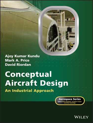
The best way to model a continuum (i.e. densely packed) airflow is to consider the medium to be composed of very fine spheres of the molecular scale (i.e. diameter 3 × 10⁻⁸ cm and intermolecular space 3 × 10⁻⁶ cm). Like sand, these spheres flow one over another, offering friction in between while colliding with one another. Air flowing over a rigid surface (i.e. acting as a flow boundary) will adhere to it, losing velocity; that is, there is a depletion of kinetic energy of the air molecules as they are trapped on the surface, regardless of how polished it may be. On a molecular scale, the surface looks like the crevices shown in Figure 3.1a, with air molecules trapped within to stagnation. The contact air layer with the surface adheres and it is known as the ‘no‐slip’ condition. The next layer above the stagnated no‐slip layer slips over it – and, of course, as it moves away from the surface, it will gradually reach the airflow velocity. The pattern within the boundary layer flow depends on how fast it is flowing.
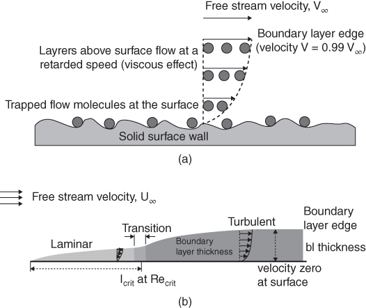
Figure 3.1 Boundary layer. (a) Magnified view of airflow over a rigid surface (boundary). (b) Boundary layer over a flat plate with a sharp leading edge.
Here is a good place to define the parameter called the Reynolds Number (Re) given in Equation 3.1. Re is a useful and powerful parameter – it provides information on the flow status with the interacting body involved.
Re increases with length.
where μ∞ = coefficient of viscosity.
It represents the degree of skin friction depending on the property of the fluid. The subscript infinity, ∞, indicates the condition, that is, undisturbed infinite distance ahead of the object. Re is a grouped parameter, which reflects the effect of each constituent variable, whether they vary alone or together. Therefore, for a given flow, characteristic length, l, is the only variable in Re. Re increases along the length. In an ideal flow (i.e. inviscid approximation), Re becomes infinity – not much information is conveyed beyond that. However, in real flow with viscosity, it provides vital information: for example, on the nature of flow (turbulent or laminar), on separation and on many other characteristics.
Figure 3.1b describes a boundary layer of airflow over a flat surface (i.e. plate) with sharp leading edge (LE) aligned to the flow direction (i.e. x‐axis). Initially, when the flow encounters the flat plate at the LE, it develops a boundary layer that keeps growing thicker until it arrives at a critical length, when flow characteristics then make a transition and the profile thickness suddenly increases. The friction effect starts at the LE and flows downstream in an orderly manner, maintaining the velocity increments of each layer as it moves away from the surface – much like a sliding deck of cards (in lamina). This type of flow is called a laminar flow. Surface skin friction depletes the flow energy transmitted through the layers until at a certain distance (i.e. the critical point) from the LE, flow can no longer hold an orderly pattern in lamina, breaking down and creating turbulence. The boundary layer thickness is shown as δ at a height where 99% of the free streamflow velocity is attained.
The region where the transition occurs is called the critical point. It occurs at a predictable distance lcrit from the LE, having a critical Re of Recrit at that point. At this distance along the plate, the nature of the flow makes the transition from laminar to turbulent flow, when eddies of the fluid mass randomly cross the layers. Through mixing between the layers, the higher energy of the upper layers energises the lower layers. The physics of turbulence that can be exploited to improve performance (e.g. dents on a golf ball forces a laminar flow to a turbulent flow) is explained later.
With turbulent mixing, the boundary layer profile changes to a steeper velocity gradient and there is a sudden increase in thickness, as shown in Figure 3.2. For each kind of flow situation, there is a Recrit. As it progresses downstream of lcrit, the turbulent flow in the boundary layer is steadily losing its kinetic energy to overcome resistance offered by the sticky surface. If the plate is long enough, then a point may be reached where further loss of flow energy would fail to negotiate the surface constraint and would leave the surface as a separated flow. Separation also can occur early in the laminar flow.

Figure 3.2 Viscous effect of air on flat plate (Cf is defined next).
The extent of velocity gradient, du/dy, at the boundary surface indicates the tangential nature of the frictional force; hence, it is shear force. At the surface where u = 0, du/dy is the velocity gradient of the flow at that point. If F is the shear force on the surface area, A, is due to friction in fluid, then shear stress is expressed as follows:
μ = 1.789 × 10⁻⁵ kg m−1 s−1 or Ns m−2 (1 g m−1 s−1 = 1 P) for air at sea level ISA.
Kinematic viscosity, ν = μ/ρm2/s (1 m2 s−1 = 104 St), where ρ is density of fluid.
The measure of the frictional shear stress is expressed as a coefficient of friction, Cf, at the point:
Friction drag for the length l, Df = ![]() (τ varies along the length).
(τ varies along the length).
Average coefficient of friction, CF is computed for a flat plate of unit length for the length l, that is, over the area (1 × l) is expressed as

The difference of du/dy between laminar and turbulent flow is shown in Figure 3.2; the latter has a steeper gradient – hence, it has a higher Cf . The up arrow indicates increase and vice versa; for incompressible flow, temp↑ makes μ↓, which reads as viscosity decreases with a rise in temperature, and for compressible flow, temp↑ makes μ↑.
The pressure gradient along flat plate gives dp/dx = 0. Airflow over curved surfaces accelerates or decelerates depending on which side of the curve the flow is negotiating (dp/dx ≠ 0). Extensive experimental investigations on the local skin friction coefficient, Cf, and IF on a 2D flat plate are available for a wide range of Re (Figure 11.22). The overall coefficient of skin friction over a surface is expressed as CF and is higher than the 2D flat plate. Cf increases from laminar to turbulent flow, as can be seen from the increased boundary layer thickness. Correction is applied to flat plate Cf , and CF to get curved surface Cf and CF. In general, CF is computed semi‐empirically from the flat plate Cf (see Chapter 11).
For flat plate in zero pressure gradient the boundary layer thickness, δ and local skin friction Cf can be expressed as given in Table 3.1 [2].
Table 3.1 Boundary layer thickness, δ, and local skin friction, Cf.
| Laminar | Turbulent | ||
| Boundary layer thickness, δ |  |
(3.5a) | |
| Local skin friction Cf |  |
 |
(3.5b) |
It is recommended to use test values as presented in graphic form in Figure 11.24. These graphs are readily available in many publications.
Scientists have been able to model the random pattern of turbulent flow using statistical methods. However, at the edges of the boundary layer, the physics is unpredictable. This makes accurate statistical modelling difficult, with eddy patterns at the edge extremely unsteady and the flow pattern varying significantly. It is clear why the subject needs extensive treatment.
To explain the physics of drag of 3D body, the classical example of flow past a sphere is shown in Figure 3.3. A sphere in inviscid flow will have no drag (Figure 3.3 ‐ left) because it has no skin friction and there is no pressure difference between the front and aft ends there is nothing to prevent the flow from negotiating the surface curvature. Diametrically opposite to the front stagnation point is a rear stagnation point, equating forces on the opposite sides. This ideal situation does not exist in nature but can provide important information.

Figure 3.3 Air flow past a sphere. (a) Inviscid flow (p1 = p2). (b) Viscous flow (p1 > p2). (c) Dented surface (p1 > p2).
In the case of a real fluid with viscosity, the physics changes nature offering drag as a combination of skin friction and the pressure difference between fore and aft of the sphere. At low Re, the low‐energy laminar flow near the surface of the smooth sphere (Figure 3.3 ‐ centre) separates early, creating a large wake in which the static pressure, p, at the aft (subscript ‘2’) cannot recover to its initial value at the front of the sphere (subscript ‘1’). The pressure at the front is now higher at the stagnation area, resulting in a pressure difference that appears as pressure drag. It would be beneficial if the flow was made turbulent by denting the sphere surface (Figure 3.3 ‐ right). In this case, high‐energy flow from the upper layers mixes randomly with flow near the surface, reenergising it. This enables the flow to overcome the spheres curvature and adhere to a greater extent, thereby reducing the wake. Therefore, a reduction of pressure drag compensates for the increase in skin friction drag (i.e. Cf increases from laminar to turbulent flow). This concept is applied to golf ball design (i.e. low Re, low velocity and small physical dimension). The dented golf ball would go farther than an equivalent smooth golf ball due to reduced drag.
The situation changes drastically for a body at high Re (i.e. high velocity and/or large physical dimension; for example, an aircraft wing or even a golf ball hit at a very high‐speed that would require more than any human effort), when flow is turbulent almost from the LE. A streamlined aerofoil shape does not have the highly steep surface curvature over large area like that of a dent less golf ball; therefore, separation occurs very late, resulting in a thin wake. Therefore, pressure drag is low. The dominant contribution to drag comes from skin friction, which can be reduced if the flow retains laminarisation over more surface area (although it is not applicable to a golf ball). Laminar aerofoils have been developed to retain laminar flow characteristics over a relatively large part of the aerofoil. These aerofoils are more suitable for low‐speed operation (but Re higher than the golf ball application) such as gliders and have the added benefit of a very smooth surface made of composite materials.
Clearly, the drag of a body depends on its profile that is, how much wake it creates. The blunter the body, the greater the wake size will be; it is for this reason that aircraft components are streamlined. This type of drag is purely viscous‐dependent and is termed profile drag. In general, in aircraft applications, it is also called parasite drag, as explained in Chapter 11.
3.3.1 Aerofoils
Aerofoils (Figure 3.4) are the 2D bread‐slice like sections of the plane wing with a streamlined geometrical shape to generate the least drag for the desired lift generated. Compared with a cylinder of a diameter equal to the maximum thickness of a well‐designed symmetrical aerofoil, the former generates 10 times more drag. A 2D flat plate of the same height placed normal to the same airflow generates 16.7 times more drag than the aerofoil. Even 3D bodies like the fuselage, nacelle and so on, are made to streamlined shapes as drag reduction measures.
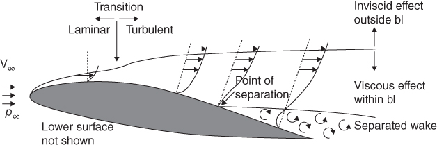
Figure 3.4 Air flow past an aerofoil.
3.4 Flow Past an Aerofoil
A typical airflow past an aerofoil is shown in Figure 3.4 later.
In Figure 3.4, the front curvature of the aerofoil causes the flow to accelerate with the associated drop in pressure, until it reaches the point of inflection on the upper surface of the aerofoil. This is known as a region of favourable pressure gradient because the lower pressure downstream favours airflow. Past the inflection point, airflow starts to decelerate, recovering the pressure (i.e. flow in an adverse pressure gradient) that was lost while accelerating. For inviscid flow, it would reach the trailing edge (TE), regaining the original free stream flow velocity and pressure conditions. In reality, the viscous effect depletes flow energy, preventing it from regaining the original level of pressure. Along the aerofoil surface, airflow depletes its energy due to friction (i.e. the viscous effect) of the aerofoil surface. The viscous effect appears as a wake behind the body.
The result of a loss of energy while flowing past the aerofoil surface is apparent in adverse pressure gradient; it is like climbing uphill. A point may be reached where there is not enough flow energy left to encounter the adverse nature of the downstream pressure rise – the flow then leaves the surface to adjust to what nature allows. Where the flow leaves the surface is called the point of separation, and it is critical information for aircraft design. When separation happens over a large part of the aerofoil, it is said that the aerofoil has stalled because it has lost the intended pressure field. Generally, it happens on the upper surface; in a stalled condition, there is a loss of low‐pressure distribution and, therefore, a loss of lift. This is an undesirable situation for an aircraft in flight. There is a minimum speed below which stalling will occur in every winged aircraft. The speed at which an aircraft stalls is known as the stalling speed, Vstall. At stall, an aircraft cannot maintain altitude and can even become dangerous to fly; obviously, stalling should be avoided.
For a typical surface finish, the magnitude of skin friction drag depends on the nature of the airflow. Below Recrit, laminar flow has a lower skin friction coefficient, Cf, and, therefore, a lower friction (i.e. lower drag). The aerofoil LE starts with a low Re and rapidly reaches Recrit to become turbulent. Aerofoil designers must shape the aerofoil LE to maintain laminar flow as much as possible.
Aircraft surface contamination is an inescapable operational problem that degrades surface smoothness, making it more difficult to maintain laminar flow. As a result, Recrit advances closer to the LE. For high‐subsonic flight speed (high Re), the laminar flow region is so small that flow is considered fully turbulent.
This section points out that designers should maintain laminar flow as much as possible over the wetted surface, especially at the wing LE. As mentioned previously, gliders – which operate at a lower Re – offer a better possibility to deploy an aerofoil with laminar flow characteristics. The low annual utilisation in private usage favours the use of composite material, which provides the finest surface finish. However, although the commercial transport wing may show the promise of partial laminar flow. With six degrees of freedom in body axes FB laminar flow at the LE, the reality of an operational environment at high utilisation does not guarantee adherence to the laminar flow. For safety reasons, it would be appropriate for the governmental certifying agencies to examine conservatively the benefits of partial laminar flow. This book considers the fully turbulent flow as starting from the LE of any surface of a high‐subsonic aircraft.
3.5 Generation of Lift
Figure 3.5a is a qualitative description of the flow field and its resultant forces on the aerofoil. The result of skin friction is the drag force, shown in Figure 3.5b. The lift is normal to the flow.

Figure 3.5 Flow field around an aerofoil. (a) Streamline pattern over aerofoil. (b) Resultant force on an aerofoil.
Section 3.8.1 explains that a typical aerofoil has an upper surface more curved than the lower surface, which is represented by the camber of the aerofoil. Even for a symmetrical aerofoil, the increase in the angle of attack increases the velocity at the upper surface and the aerofoil approaches stall, a phenomenon described in Section 3.4.
Figure 3.6a shows the pressure field around the aerofoil. The pressure at every point is given as the pressure coefficient distribution, as shown in Figure 3.6b. The upper surface has lower pressure, which can be seen as a negative distribution. In addition, cambered aerofoils have moments that are not shown in the figure.
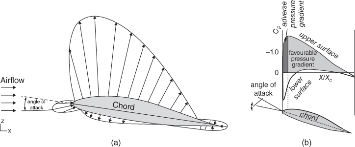
Figure 3.6 Pressure field representations around an aerofoil. (a) Pressure field distribution. (b) Cp distribution over an aerofoil.
Figure 3.7a shows flow physics around the aerofoil. At the LE, the streamlines move apart: One side negotiates the higher camber of the upper surface and the other side negotiates the lower surface. The higher curvature at the upper surface generates a faster flow than the lower surface. They have different velocities when they meet at the TE, creating a vortex sheet along the span. The phenomenon can be decomposed into a set of straight streamlines representing the free streamflow condition and a set of circulatory streamlines of a strength that matches the flow around the aerofoil. The circulatory flow is known as the circulation, γ, of the aerofoil (Figure 3.7b). The concept of circulation provides a useful mathematical formulation to represent lift. Circular flow is generated by the effect of the aerofoil camber, which gives higher velocity over the upper wing surface. The directions of the circles show the increase in velocity at the top and the decrease at the bottom, simulating velocity distribution over the aerofoil.
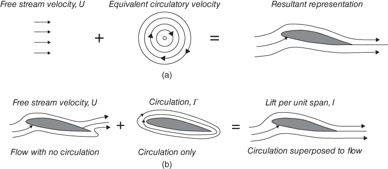
Figure 3.7 Lift generation on an aerofoil. (a) Mathematical representation by superimposing free vortex flow over parallel flow. (b) Inviscid flow representation of flow around an aerofoil.
The flow over an aerofoil develops a lift per unit span of l = ρUγ (see other textbooks [2–7] for the derivation). Computation of circulation is not easy. This book uses accurate experimental results to obtain the lift.
3.6 Aircraft Motion, Forces and Moments
An aircraft is a vehicle in motion; in fact, it must maintain a minimum speed above the stall speed. The resultant pressure field around the aircraft body (i.e. wetted surface) is conveniently decomposed into a usable form for designers and analysts. The pressure field alters with changes in speed, altitude and orientation (i.e. attitude). This book primarily addresses a steady level flight pressure field; the unsteady situation is considered transient in manoeuvres. Chapter 17 addresses certain unsteady cases (e.g. gusty winds) and references are made to these design considerations when circumstances demand it. This section provides information on the parameters concerning motion (i.e. kinematics) and force (i.e. kinetics) used in this book.
3.6.1 Motion
Unlike an automobile, which is constrained by the road surface, an aircraft is the least constrained vehicle, having all the degrees of freedom (Figure 3.8): three linear and three rotational motions along and about the three axes. These can be represented in any coordinate system; however, in this book, the right‐handed Cartesian coordinate system is used. Controlling motion in six degrees of freedom is a complex matter. Careful aerodynamic shaping of all components of an aircraft is paramount, but the wing takes top priority. Aircraft attitude is measured using Eulerian angles – ψ (azimuth), θ (elevation) and Φ (bank) – and these are in demand for aircraft control; however, this is beyond the scope of this book. In classical flight mechanics, many types of Cartesian coordinate systems are in use. The three most important are as follows:
- Body‐fixed axes, FB, is a system with the origin at the aircraft centre of Gravity (CG) and the x‐axis pointing forward (in the plane of symmetry), the y‐axis going over the right wing, and the z‐axis pointing downward.
- Wind‐axes system, FW, also has the origin (gimballed) at the CG and the x‐axis aligned with the relative direction of airflow to the aircraft and points forward. The y‐ and z‐axes follow the right‐handed system. Wind axes vary, corresponding to the airflow velocity vector relative to the aircraft.
- Inertial axes, FI, fixed on the Earth. For speed and altitudes below Mach 3 and 100 000 ft., respectively, the Earth can be considered flat and not rotating, with little error, so the origin of the inertial axes is pegged to the ground. Conveniently, the x‐axis points north and the y‐axis east, making the z‐axis point vertically downwards in a right‐handed system.
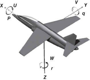
Figure 3.8 Six degrees of freedom in body axes.
In a body‐fixed coordinate system, FB, the components of six degrees of freedom are as follows:
| Linear velocities | U along x‐axis (+ve forward) |
| V along y‐axis (+ve right) | |
| W about z‐axis (+ve down) | |
| Angular velocities | p about x‐axis known as roll (+ve) – aileron activated |
| q about y‐axis known as pitch (+ve nose up) – elevator activated | |
| r about z‐axis known as yaw (+ve) – rudder activated | |
| Angular acceleration | |
In the wind‐axes system, FW, the components of six degrees of freedom are as follows:
| Linear velocities | V along x‐axis (+ve forward) |
| Linear accelerations | |
| and so on. |
If the parameters of one coordinate system are known then parameters in other coordinate system can be found out through transformation relationship.
3.6.2 Forces
In a steady‐state level flight, an aircraft is in equilibrium under the applied forces (i.e. lift, weight, thrust and drag) as shown in Figure 3.9. Lift is measured perpendicular to aircraft velocity (i.e. free stream flow) and drag is opposite to the direction of aircraft velocity (naturally, the wind axes, FW, are suited to analyse these parameters). In a steady level flight, lift and weight are opposite one another; opposite forces may not be collinear.

Figure 3.9 Equilibrium flight (CG at ⊕) (Folland Gnat: the 1960s, United Kingdom – world's smallest fighter aircraft. Fuselage length = 9.68 m, span = 7.32 m, height = 2.93 m).
In steady level flight (equilibrium, un‐accelerated flight), the aircraft weight is exactly balanced by the lift produced by the wing (fuselage and other bodies could share a small part of lift – to be discussed later). Thrust provided by the engine is required to overcome drag.
It gives ∑ Force = 0,
That is, in vertical direction, lift (L) = weight (W) and in horizontal direction, thrust (T) = drag (D).
in short:
that is, in equilibrium the vertical direction, lift = weight, and in the horizontal direction, thrust = drag. The aircraft weight is exactly balanced by the lift produced by the wing (the fuselage and other bodies could share a part of the lift – discussed later). Thrust provided by the engine is required to overcome drag.
3.6.3 Moments
The forces are not necessarily collinear and also the components of an aircraft have their inherent moments. Moments arising from various aircraft components are summed to zero to keep in straight flight, that is, in steady level flight ∑ Moment = 0.
Any force/moment imbalance would show up in the aircraft flight profile. This is how an aircraft is manoeuvred – through force and/or moment imbalance – even for the simple actions of climb and descent.
When not in equilibrium the accelerating forces are taken into account at the instant of computation to find its resultant affecting aircraft flight condition. If there were any force/moment imbalance, it would show up in the aircraft flight profile. That is how an aircraft is manoeuvred – through force and/or moment imbalance – even for simple actions of climb and descent.
A summary of forces and moments in body axes FB is tabulated in Table 3.2.
Table 3.2 Aircraft forces and moments in body frame, FB.
| Axis | Force | Moment | Velocity Component | Angle | Angular Velocity Component |
| x | X | L | U | ϕ | p |
| y | Y | M | V | θ | q |
| z | Z | N | W | ψ | r |
In wind axes, FW, the forces and moments are transformed to different magnitude and direction where the force components X, Y and Z are resolved to lift (L), drag (D) and side force (C).
3.6.4 Basic Control Deflections – Sign Convention
Conventional aircraft have four basic controls: the elevators, ailerons, rudder and throttle. The elevator and the throttle are longitudinal controls, that is, they affect the two longitudinal degrees of freedom: changes of speed along the Ox‐axis and pitch about the Oy‐axis. Likewise, the ailerons and the rudder are called lateral controls because they affect the three lateral degrees of freedom: sideslip along the Oy‐axis; roll about the Ox‐axis and yaw about the Oz‐axis.
- (i) Elevator. The elevator is used to control the angle of attack of the aircraft, that is, pitch change and therefore its airspeed at constant power. This will be demonstrated when we come to the consideration of Longitudinal Static Stability. Note that positive elevator angle, η, generates negative pitching moment, M, and that this is achieved by pushing the control column forward (Figure 3.10).
- (ii) Aileron. The ailerons are used to control the aircraft in roll. More specifically, the ailerons apply a rolling moment to the aircraft and so are used to demand roll rate. Roll rate is used to achieve bank angle, and bank angle is used to initiate a turn. Note that positive aileron angle (right hand side down), ξ, generates negative rolling moment, L (Figure 3.10).
- (iii) Rudder. The rudder is used to control the side slip angle of the aircraft. This might be of turn. Note that positive rudder angle, ζ, generates negative yawing moment, N (Figure 3.10).
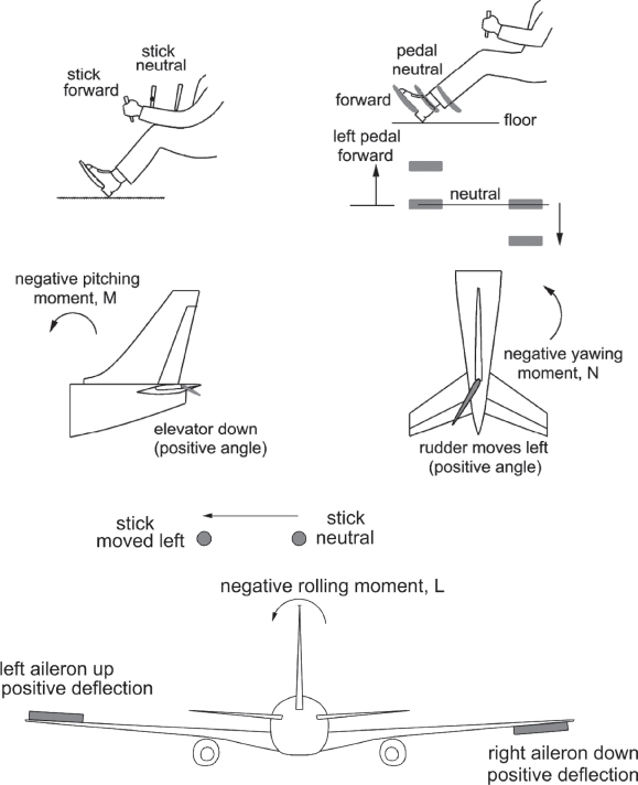
Figure 3.10 Control deflection and sign convention.
Heaving up and down results mainly from encountering sudden gust or arise as transient state of a manoeuvre.
The symbols employed to label the forces, moments and linear and angular velocities in this coordinate system are given in Table 3.1. This notation is used in flight dynamics (there are other conventions notably that are used in USA). (Note that L is used to denote the lift and V to denote the true airspeed of the aircraft. This will not cause confusion because the context will always make it clear whether, for example, L refers to lift or rolling moment.)
Heaving (whole aircraft vertical movement) in the Oz direction can occur as a result of encountering a vertical gust or as a transient state on account of control application.
3.6.5 Aircraft Loads
Chapter 17 deals with aircraft load in detail. In this section, only a preliminary definition is given to get an idea on what aircraft load means and its basic definition.
An aircraft is subject to load at any time. In flight, aircraft load varies with manoeuvres and/or when gusts are encountered. Early designs resulted in many structural failures in operation. Figure 3.11 gives the force diagram of an aircraft in accelerated flight (pull‐up).
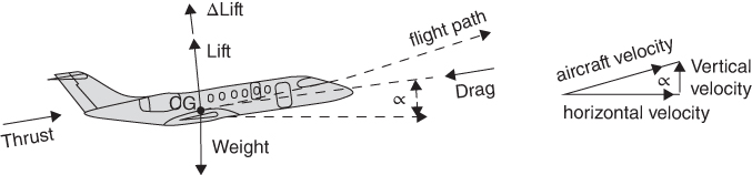
Figure 3.11 Equilibrium flight.
Newton's law states that change from an equilibrium state requires an additional applied force, that would associate with some form of acceleration, a. When applied in the pitch plane to increase the angle of incidence, α, initiated by rotation of the aircraft, the additional force appears as an increment in lift, ΔL, resulting in gain in height (Figure 3.11).
The load factor, n, indicates the increase in force contributed by the centrifugal acceleration, a. The load factor, n = 2, indicates a two‐fold increase in weight; that is, a 90‐kg person would experience a 180‐kg weight. The load factor, n, is loosely termed as the g load; in this example, it is the 2‐g load.
3.7 Definitions of Aerodynamic Parameters
Section 3.4 has already given the definition of Re and described the physics of the laminar/turbulent boundary layer. This section gives other useful non‐dimensional coefficients and derived parameters frequently used in this book. The most common nomenclature, without any conflicts between both the sides of Atlantic are listed here – these are internationally understood.
(subscript ∞ represents free stream condition and is sometimes dropped)
‘q’ is a parameter extensively used to non‐dimensionalise lumped parameters.
The coefficients of 2D aerofoil and 3D wing differ as shown next (lower case subscripts represent the 2D aerofoil and the capital letters are for the 3D wing).
- Cl = sectional aerofoil lift coefficient = section lift/qc
- Cd = sectional aerofoil drag coefficient = section drag/qc
- Cm = aerofoil pitching moment coefficient = section pitching moment/qc2 (+ nose up)
3.12

- CL = lift coefficient = lift/qSW
- CD = drag coefficient = drag/qSW
- CM = pitching moment coefficient = lift/qSW2 (+ nose up)
Chapter 4 deals with 3D wings, where correction to 2D results necessarily arrives at 3D values. The next section deals with lift generation over an aerofoil and pressure distribution in at any point over the surface in terms of pressure coefficient, Cp, which is defined as:
Equation (1.4) defined pressure coefficient at a point as,
Then sectional lift coefficient Cl of an aerofoil can be expressed as
3.8 Aerofoils
The cross‐sectional shape of a wing (i.e. the bread‐slice‐like sections of a wing comprising the aerofoil) is the crux of aerodynamic considerations. The wing is a 3D surface (i.e. span, chord and thickness). An aerofoil represents 2D geometry (i.e. chord and thickness). Aerofoil characteristics are evaluated at mid‐wing to eliminate the finite 3D wing tip effects. Typically, its characteristics are expressed over unit chord permitting scaling to fit any suitable size.
Aircraft performance depends on the type of aerofoil incorporated in its wing design. Aerofoil design is a specialised topic not dealt with in this book. There are many well proven existing aerofoils catering for a wide range of performance demands. NACA/NASA have systematically developed aerofoils in a family of designs and these are widely used by many aircraft. The majority of general aviation (GA) aircraft have NACA aerofoils. However, to stay ahead of competition, all major aircraft manufacturers develop their own aerofoils that are kept ‘commercial in confidence’ as proprietary information. These are not available in public domain. Moreover, unless these aerofoils can be compared it is not recommended to use them in undergraduate studies. The NACA series aerofoil will prove sufficient to make a good GA aircraft and this book only depends on this family.
Nowadays, there are specialised application software packages for designing aerofoil sections and these can bring out credible results. The only way to apply them is to verify the analytical results by comparing with wind tunnel test results. Certification of any new aerofoil is an additional task.
This section introduces various types of aerofoil and their geometrical characteristics. Subsequent chapters deal with aerofoil characteristic and how to make the selection. The 3D effects of a wing are discussed in Section 4.7.
3.8.1 Subsonic Aerofoils
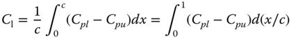
To standardise aerofoil geometry, Figure 3.12 provides the universally accepted definitions that should be well understood [6].
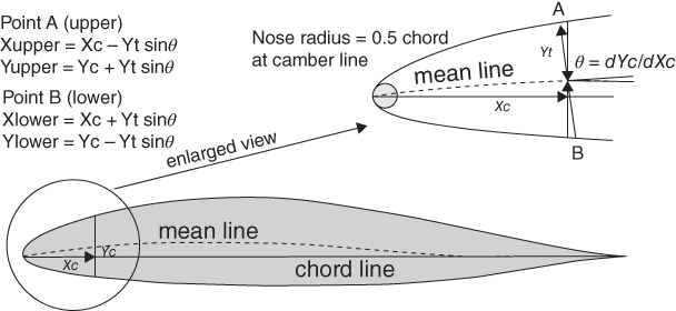
Figure 3.12 Aerofoil section and definitions – NACA family.
Chord length is the maximum straight‐line distance from the LE to the TE. The mean line represents the mid‐locus between the upper and lower surfaces. The camber of an aerofoil is expressed as the percent deviation of the mean line from the chord line. The mean line is known as the camber line. Coordinates of the upper and lower surfaces are denoted by yU and xL for the distance measured from the chord line.
The chord line is kept aligned to the x‐axis of the Cartesian coordinate system and measured from the LE. The thickness (t) of an aerofoil is the distance between the upper and the lower contour lines at the distance along the chord, measured perpendicular to the mean line and expressed in percentage of the full chord length. Conventionally, it is expressed as the thickness to chord (t/c) ratio as a percentage. A small radius at the LE is necessary to smooth out the aerofoil contour. It is convenient to present aerofoil data with the chord length non‐dimensionalised to unity so that the data can be applied to any aerofoil size.
Aerofoil pressure distribution is measured in a wind tunnel (also in CFD) to establish its characteristics, as shown in [6]. Wind tunnel tests are conducted at mid‐span of the wing model so that results are as close as possible to 2D characteristics. These tests are conducted at several Re values. A higher Re indicates a higher velocity; that is, it has more kinetic energy to overcome the skin friction on the surface, thereby increasing the pressure difference between the upper and lower surfaces and, hence, more lift.
3.8.2 Aerofoil Lift Characteristics
Figure 3.13 shows the typical test results of an aerofoil as plotted against a variation of the angle of attack, α. These graphs show aerofoil characteristics.
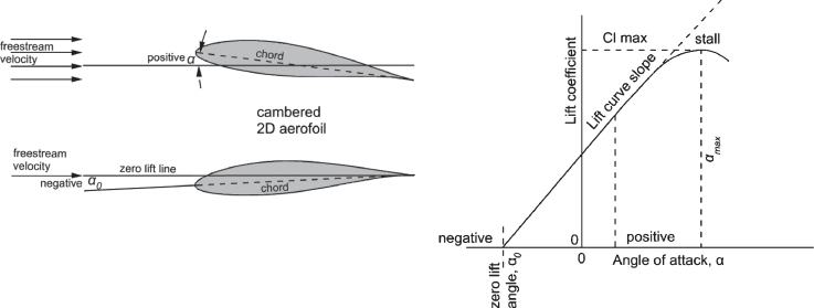
Figure 3.13 Typical aerofoil characteristics.
Angle between free stream velocity vector aerofoil is the angle of attack, α. As α increases, the upper curvature effect increases over the aerofoil airflow velocity, thereby increasing circulation that results in generating more lift up to a point when viscous effects deplete flow energy to make the aerofoil stall as explained in Section 3.5. This is shown in Figure 3.13: that until the incipient stage of stall the lift increases, it varies linearly with α increase. This is the operating range of aircraft at α well below the incipient stage of stall. A cambered aerofoil develops some lift at α = 0. In this case, the zero lift angle α0 is negative. Initially, the variation is linear; then, at about 8° to 10° α, it starts to deviate reaching maximum Clmax at αmax. Past αmax, the Cl drops rapidly – if not drastically – when stall is reached. Stalling starts at reaching αmax. The lift curve slope dCl/dα is slope of the lift curve within its linear range of variation, typically measured between α from about −2° to 6°.
3.8.3 Groupings of Subsonic Aerofoils – NACA/NASA
From the early days, European countries and the United States undertook intensive research to generate better aerofoils to advance aircraft performance. By the 1920s, a wide variety of aerofoils appeared and consolidation was needed. Since the 1930s, NACA generated families of aerofoils benefiting from what was available in the market and beyond by further testing. It presented the aerofoil geometries and test results in a systematic manner, grouping them into family series. The generic pattern of the NACA aerofoil family is listed in [6] with well‐calibrated wind tunnel results. The book was published in 1949 and has served aircraft designers (civil and military) for more than half a century and is still useful. The NACA was subsequently reorganised to the NASA and continued with aerofoil development, concentrating on having better laminar flow characteristics over an aerofoil. Also, the industry undertook research and development to generate better aerofoils for specific purposes, but they are kept ‘commercial in confidence’.
Designations of the NACA series of aerofoils are as follows: four‐, five‐ and six‐digit, given here are the ones of the interest to this book. Many fine aircraft have used the NACA aerofoil. However, brief comments on other types of aerofoil are also included.
The NACA four‐ and five‐digit aerofoils were created by superimposing a simple camber‐line shape with a thickness distribution that was obtained by fitting with the following polynomial [6]:
3.8.3.1 NACA Four‐Digit Aerofoil
Each of the four digits of the nomenclature represents a geometrical property, as explained here using the example of the NACA 2315 aerofoil, is shown in Figure 3.14.

Figure 3.14 Camber‐line distribution of the NACA 2315.
| 2 | 3 | 15 |
| Maximum camber, yc as a percentage of chord | Location of yc‐max in 1/10 of chord from the LE ratio as a percentage of chord | The last two digits give the maximum thickness to the chord |
The camber line of four‐digit aerofoil sections is defined by a parabola from the LE to the position of maximum camber followed by another parabola to the TE (Figure 3.14). This constraint did not allow the aerofoil design to be adaptive. For example, it prevented generation of aerofoil with more curvature towards the LE in order to provide better pressure distribution. Figure 3.15 compares NACA 0015, NACA 4412 and NACA 4415 geometries.
Figure 3.15 Comparing NACA 0015, NACA 4412 and NACA 4415 geometries.
3.8.3.2 NACA Five‐Digit Aerofoil
After the four‐digit sections came the five‐digit sections. The first two and last two digits represent the same definitions as the four‐digit NACA aerofoil and are still applicable except the camber shape differs as defined by the middle digit. The middle digit stands for the aft position of the mean line bringing the change in defining camber‐line curvature. The middle digit has only two options of zero for a straight (i.e. standard) and one for an inverted cube. These are explained next for the NACA 23012 with NACA 23112 aerofoil.
| 2 | 3 | 0 or 1 | 12 |
|
Maximum camber as a percentage of chord, YC The design‐lift coefficient is 3/2 of it, in tenths |
Max. thickness of max camber in 1/20 of chord XC |
0 – straight/standard 1 – inverted cube |
The last two digits give the maximum thickness to chord ratio as a percentage of chord |
3.8.3.2.1 Explanation for NACA 23012
- First digit, 2. It has 0.02c maximum amount of camber with design‐lift coefficient = 2 × (3/20) = 0.3.
- Second digit, 3. Position of maximum camber at 3 × 2/200 = 15% chord length from LE.
- Third (middle) digit 0. Aft camber shape is straight (standard).
- Last two digits, 12. It has maximum thickness to chord ratio = 0.12, i.e. 12% of the chord length.
NACA 23112: Same as before, except that its aft camber shape has a inverted cube shape; that is, curved (NACA Report 537]. Figure 3.16 compares the NACA 23012 with the NACA 23112 aerofoil.
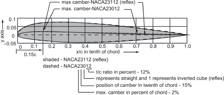
Figure 3.16 Comparison of an NACA 23012 aerofoil with NACA 23112 reflex aerofoils.
The NACA five series have been well used in many GA/utility category aerofoil. They have higher Clmax, low Cm‐ac with good Cdmin and Clα. However, these aerofoils are not suitable for ab nitio trainer aircraft due to abrupt stall characteristics that are not forgiving for student pilots.
3.8.3.3 NACA Six‐Digit Aerofoil
The five‐digit family was an improvement over the four‐digit NACA series aerofoil; however, researchers subsequently found better geometric definitions to represent a new family of a six‐digit aerofoil. The state‐of‐the‐art for a good aerofoil often follows reverse engineering – that is, it attempts to fit a cross‐sectional shape to a given pressure distribution. The NACA six‐digit series aerofoil came much later (it was first used for the P51 Mustang design in the late 1930s) from the need to generate a desired pressure distribution instead of being restricted to what the relatively simplistic four and five‐digit NACA series could offer. The six‐digit series aerofoils were generated from a more or less prescribed pressure distribution and were designed to achieve some laminar flow. This was achieved by placing the maximum thickness far back from the LE. Their low‐speed characteristics behave like the four‐ and five‐digit series but show much better high‐speed characteristics. However, the drag bucket seen in wind tunnel test results may not show up in actual flight. Some six‐digit aerofoils are more tolerant to production variation compared to typical five‐digit aerofoils.
NACA six‐digit aerofoils are possibly those most popular, widely used in various classes of aircraft. Their success was followed by increased effort to develop an aerofoil with laminar flow characterises over a wide speed regime. The definition for the NACA six‐digit aerofoil example using NACA 632‐212 is as follows.
An NACA six‐digit aerofoil example 632‐212 definition is:
| 6 | 3 | Subscript 2− | 2 | 12 |
| Six Series | Location of min Cp in 1/10 chord | Half width of low drag bucket in 1/10 of Cl |
Ideal Cl in tenths (design) |
Max thickness as a percentage of chord |
The six‐digit aerofoil nomenclature follows the following sequence.
- first number. The number ‘6’ indicating the series.
- *second number. One digit describing the distance of the minimum cp (pressure) area in tens of percentage points of the chord.
- **third number. The subscript digit gives the range of lift coefficient in tenths above and below the design‐lift coefficient in which favourable pressure gradients exist on both surfaces.
- A hyphen in between.
- fourth number. Ideal aerofoil design‐lift coefficient Cl in tenths.
- fifth and sixth numbers. The last two digits is the maximum thickness as a percentage of the chord.
- *It does not refer to camber. In the complete form, the six series mean line type is indicated by an associated letter ‘a’ (p. 121 of [6]), not given here.
- **The subscript can also be expressed in parentheses, for example 632‐212 as 63(2)‐212. Within the parentheses there could be more numbers as explained in [6]. A modified aerofoil can carry the letter ‘A’ (e.g. 641A212 given in p. 122 of [6].
The nomenclature of NACA six series is an involved one. The readers are recommended to refer to [1] (section 3.8 and p. 119–122) for the exact definition. This book only covers how to use the graphs of the extent applied in worked‐out examples.
In the example of the six‐series aerofoil NACA 652‐415 given in Figure 3.17, the minimum pressure position is at the 50% chord location indicated by the second digit. This is the point of inflection at the upper surface. The subscript 2 indicates that the minimum drag coefficient (drag bucket) is near its minimum value over a range of Cl of 0.2 above and below the design‐lift coefficient. The next digit indicates the design‐lift coefficient of 0.4, and the last two digits indicate the maximum thickness in percentage of the chord of 15%.
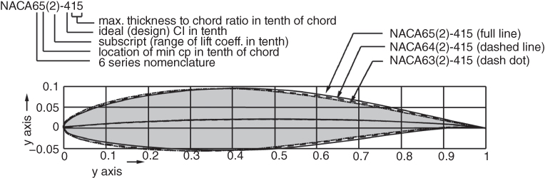
Figure 3.17 Comparison of NACA652 415, NACA642 415 and NACA632 415 aerofoils.
Three NACA six‐series aerofoils are compared with location of minimum Cp from 0.3c to 0.5c from the LE.
3.8.3.4 NACA Seven‐Digit Aerofoil
The seven‐digit family of aerofoil followed to further maximising laminar flow achieved by separately identifying the low‐pressure zones on upper and lower surfaces of the aerofoil. The aerofoil is described by seven digits in the following sequence (Figure 3.18).
- first number. The number ‘7’ indicating the series.
- second number. One digit describing the distance of the minimum pressure (Cp) area on the upper surface in tens of percent of the chord.
- third number. One digit describing the distance of the minimum pressure area on the lower surface in tens of percent of the chord.
- fourth is one letter referring to a standard profile from the earlier NACA series.
- fifth number. Single digit describing the lift coefficient in tenths.
- sixth and seventh number. The last two digits give the maximum thickness as a percentage of the chord.
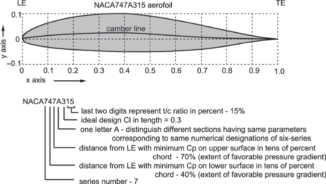
Figure 3.18 The Seven Series NASA747A315 aerofoil.
Figure 3.18 is an example of the NACA 747A315 of the seven‐digit aerofoil series. The first digit ‘7’ indicates the series number. The second digit ‘4’ signifies that it has favourable pressure gradient on the upper surface to the extent of 40% of chord peaking to minimum cp and thereafter starts the adverse pressure gradient. The third digit ‘7’ says the same for the lower surface and in this case up to 70%. The last three digits are same nomenclature as for the six‐digit NACA aerofoil, indicating it has a design‐lift coefficient of Cl = 0.3 and a maximum thickness of 15% of the chord, preceded by a letter ‘A’ to distinguish that it has a class of different sections.
3.8.3.5 NACA Eight‐Digit Aerofoil
The NACA eight‐digit aerofoil series are the supercritical aerofoils designed to independently maximise airflow above and below the wing. These are a variation of the six‐series and seven‐series and the eight‐digit series has the same numbering system as the seven‐series aerofoils except that the first digit is an ‘8’ to identify the series. Application of NACA eight‐digit aerofoils to aircraft is yet to be proven and not discussed here.
3.8.3.6 Peaky‐Section Aerofoil
Peaky‐section aerofoils were developed during the early 1960s by the large commercial aircraft manufacturers to fly at higher Mcrit (20 count drag rise – see Section 3.14). It was done by tweaking their well‐proven high performing aerofoil of the time by slightly drooping down the aerofoil nose section and re‐contouring. This allowed a rise of local airspeed near the LE on account well designed nose droop, causing negative Cp to peak up, hence the name (Figure 3.19). Distributed weak local shocks were allowed to form at that area that do not cause flow separation until it may happen further downstream when higher Mcrit is reached.

Figure 3.19 Comparison between a peaky‐section aerofoil with a conventional aerofoil.
The NASA supercritical aerofoil appeared during the mid‐1960s and gradually replaced the peaky‐section aerofoil.
3.8.3.7 NASA Supercritical Aerofoil
In an effort to develop aerofoil to operate at a higher subsonic speed yet retaining good low‐speed characteristics better than what existed, Richard T. Whitcomb of the Langley Research Center developed the supercritical aerofoil during the early 1960s. The goal was to increase the drag divergence Mach number (Figure 3.14), thereby reducing drag and allowing for more efficient flight in the transonic regime. It has the characteristic shape of a flat top following a large LE radius and curved tail with thickness at the TE.
This distinctive aerofoil shape helps the local supersonic flow with isentropic recompression on account of reduced curvature over the middle region of the upper surface and substantial aft camber.
The National Aeronautics and Space Administration (NASA) made systematic studies in three phases during the 1970s to develop this family of aerofoils with thicknesses from 2 to 18% and design‐lift coefficients from 0 to 1.0. These were called the ‘supercritical aerofoils’.
Three phases of development are as follows:
- Phase 1. Supercritical Aerofoils: Early Supercritical Aerofoils that increased the drag divergence Mach number beyond the six‐series NACA family.
- Phase 2. Supercritical Aerofoils: The extension of Phase 1 Supercritical Aerofoils with target pressure distributions.
- Phase 3. Supercritical Aerofoils: aerofoils developed for studies to reduce Phase 2 LE radii. The study was eventually abandoned.
The supercritical aerofoil number designation is in the form in the example of SC(2)‐0412 as shown in Figure 3.20. The aerofoil designation is broken down into two segments – the first segment of three characters starts with SC, indicating it is a supercritical aerofoil and the bracketed number shows the development phase – in this case, Phase II of three phases of development as described next. The last segment starts with its first two digits as the design‐lift coefficient in tenths and the last two are the thickness in percent chord, in the example Cl = 0.4 and t/c = 12%.
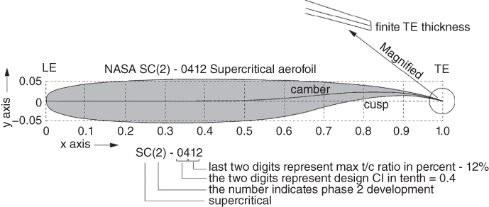
Figure 3.20 Supercritical aerofoil NASA SC(2)‐0412.
3.8.3.8 Natural Laminar Flow (NLF) Aerofoil
The NLF class of aerofoil was designed by NASA during the early 1980s as a follow‐up of the successful NACA six‐series aerofoil for low subsonic speed GA aircraft operation offering low profile drag at high Re. NLF(1)‐0213 and NLF(1)‐0414 exhibited good laminar flow up to 70% of chord length at Mach 0.4 and Re = 10 × 106. NLF type aerofoils suit the composite wing, that can have smooth polished surface, better than a metal wing.
Typically, NLF aerofoil shows ‘flat roof‐top’ pressure distribution. NLF(1)‐0414 has achieved Clmax = 1.83 at α = 18° operating at Re = 10 × 106. Figure 3.21 compares the NLF(1)‐0414 with NACA 67‐314.
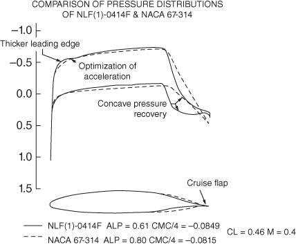
Figure 3.21 Natural laminar flow aerofoil.
Later for high‐speed applications, for example, business jets, HSNLF(1) – 0213 was designed to suit applications in compressible flow (HSNLF = high speed natural laminar flow aerofoil).
3.8.3.9 NACA GAW Aerofoil
The NASA General Aviation Wing (GAW) series evolved later for low‐speed applications and use by GA (Figure 3.22). Although the series showed better lift‐to‐drag characteristics, their performance with flap deployment, tolerance to production variation and other issues are still in question. As a result, the GAW aerofoil has yet to compete with some of the older NACA aerofoil designs. However, a modified GAW aerofoil has appeared with improved characteristics.

Figure 3.22 NASA/Langley/Whitcomb LS(2)‐0413 (GA(W)‐2) general aviation aerofoil.
The numbering system is similar to the supercritical aerofoil.
3.8.3.10 Supersonic Aerofoils
A supersonic aerofoil is a cross‐section geometry designed to generate lift efficiently at supersonic speeds (Figure 3.23). The need for such a design arises when an aircraft is required to operate consistently in the supersonic flight regime. Supersonic aerofoils are necessarily thin in the range of ≈0.04 < (t/c) < ≈0.07.
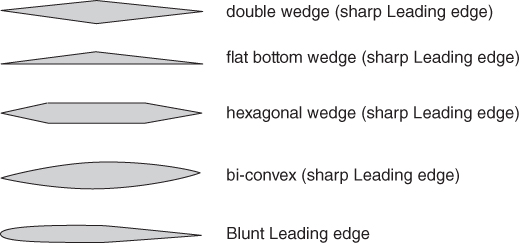
Figure 3.23 Supersonic aerofoil.
Supersonic aerofoils generally have a thin section formed of either angled planes (called ‘double wedge aerofoil’) or opposed arcs (called ‘biconvex aerofoil’) with very sharp leading and TEs. The sharp edges prevent the formation of a detached bow shock in front of the aerofoil as it moves through the air. This shape is in contrast to subsonic aerofoils, which often have rounded LEs to reduce flow separation over a wide range of angle of attack A rounded edge would behave as a blunt body in supersonic flight and thus would form a bow shock, which greatly increases wave drag. The aerofoils' thickness, camber and angle of attack are varied to achieve a design that will cause a slight deviation in the direction of the surrounding airflow.
However, since a round LE decreases an aerofoil's susceptibility to flow separation, a sharp LE implies that the aerofoil will be more sensitive to changes in angle of attack. Therefore, to increase lift at lower speeds, aircraft that employ supersonic aerofoils also use high‐lift devices such as LE and TE flaps. The thin six and seven series aerofoils have been used in combat aircraft design.
The supersonic aerofoil designation is as follows.
The letter ‘N’ is replaced by the series number, the number ‘1’ being used for wedge‐shape profiles and the number ‘2’ being used for circular arc profiles. The letter ‘S’ denotes it is supersonic. The letter ‘X1’ represents the distance along the chord from the LE to the point of maximum thickness ‘Y1’ for the upper surface. The letters ‘X2’ and ‘Y2’ represent the corresponding values for the lower surface. ‘X’ and ‘Y’ are the percentage aerofoil cord length. In the following are some examples of 6% t/c aerofoil.
| Subsonic | |
| NACA 66‐006 | blunt LE aerofoil |
| Supersonic | |
| NACA 1S‐(30)(03)‐(30)(03) | wedge shaped aerofoil (double wedge, max. thickness at 30% chord) |
| NACA 1S‐(70)(03)‐(70)(03) | |
| NACA 2S‐(30)(03)‐(30)(03) | |
| NACA 2S‐(50)(03)‐(50)(03) | circular arc aerofoil (in this case biconvex, max. thickness in middle) |
| NACA.2S‐(70)(03)‐(70)(03) |
Typically, the sharp LE thin supersonic aerofoil, at its clean basic configuration, has low Clmax (in the order of 0.8 to 0.9). Its LE droop increases the aerofoil camber giving ΔClmax in the order of 0.4 to 0.5. A 20° TE deflection can give nearly twice the Clmax of the basic aerofoil Clmax.
3.8.3.11 Other Types of Subsonic Aerofoil
NACA's earliest attempt (in the 1930s) to make a systemic generic type was the NACA 1‐Series (or 16 series) [6]. This new approach to aerofoil design had its shape mathematically derived from the desired lift characteristics. Prior to this, aerofoil shapes were first created and then had their characteristics measured in a wind tunnel. The 1‐series aerofoils are described by five digits. Since this type is no longer used, it is not discussed here.
Subsequently, after the six series sections, aerofoil design became more specialised with aerofoils designed for their particular application. In the mid‐1960s, Whitcomb's ‘supercritical’ aerofoil allowed flight with high critical Mach numbers (operating with compressibility effects, producing in wave drag) in the transonic region. The NACA seven and eight series were designed to improve some aerodynamic characteristics. In addition to the NACA aerofoil series, there are many other types of aerofoil in use.
To remain competitive, the major industrial companies generate their own aerofoil. One example is the peaky‐section aerofoil that were popular during the 1960s and 1970s for the high‐subsonic flight regime. Aerofoil designers generate their own purpose‐built aerofoil with good transonic performance, good maximum lift capability, thick sections, low drag and so on – some are in the public domain but most are held commercial in confidence for strategic reasons of the organisations. Subsequently, more transonic supercritical aerofoils were developed, by both research organisations and academic institutions. One such baseline design in the United Kingdom is the RAE 2822 aerofoil section, whereas the CAST 7 evolved in Germany. It is suggested that readers examine various aerofoil designs.
There are many other types of aerofoil, for example, Eppler, Liebeck (used in gliders) and many older types, for example, the Wortmann, Gottingen, Clark Y, Royal Air Force (RAF) aerofoils and so on, not discussed here. There are large number of other aerofoil developed by many scientists, in addition to proprietary aerofoil developed by industry. However at this stage, the well‐used and established NACA series aerofoils will serve adequately until the readers join industry to use their data and analyses methods, today using CFD. While, NACA series aerofoil test data are still prevalent, the use of DATCOM (the short name for the USAF Data Compendium for Stability and Control)/ Engineering Sciences Data Unit (ESDU) for aerofoil analyses is gradually receding. URLs [8–11] may prove useful to get some information on various types of aerofoil.
3.8.3.11.1 Discussion
In earlier days, drawing the full‐scale aerofoils of a large wing and their manufacture was not easy and great effort was required to maintain accuracy to an acceptable level; their manufacture was also not easy. Today, computer‐aided drawing/computer‐aided manufacture (CAD/CAM) and microprocessor‐based numerically controlled lofters have made things simple and very accurate. In December 1996, NASA published a report outlining the theory behind the U.S. National Advisory Committee for Aeronautics (NACA) (predecessor of the present‐day NASA) aerofoil sections and computer programs to generate the NACA aerofoil.
Aerofoil characteristics are sensitive to geometry and require hard tooling with tight manufacturing tolerances to manufacture to adhere closely to the profile.
Often, a wing design has several aerofoil sections varying along the wing span. Appendix F provides six types of aerofoil for use in this book. Readers should note that the 2D aerofoil wind tunnel test is conducted in restricted conditions and will need corrections for use in real aircraft. Section 3.15.1 gives a simplified aerofoil selection method.
3.9 Reynolds Number and Surface Condition Effects on Aerofoils – Using NACA Aerofoil Test Data
This section explains the NACA aerofoil test result that shows the Re effect. NACA aerofoil test data is compiled in a specific format [6]. Figure 3.24 gives the traced NACA 65‐410 aerofoil test data [6]. A higher Re implies higher airspeed that increases Clmax (shown magnified in Figure 3.24), assisted by increased energy of airflow.
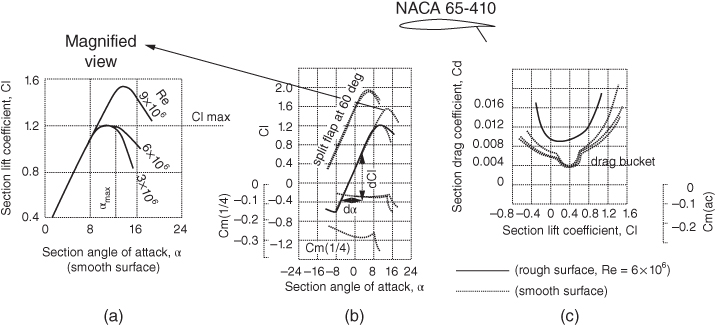
Figure 3.24 Traced NACA 65‐410 aerofoil test data at three Re values [1]. (a) Magnified graph. (b) Cl and Cm1/4 result. (c) Cd and Cm‐ac result.
A small aircraft with 4 ft chord flying at 100 mph (146.7 ft s−1) at sea level standard has Re = 3.85 × 10⁶ (μ0 = 3.62 × 10⁻⁷ lb‐sec ft−2). This will require a large wind tunnel to do the tests. To keep cost low, tests are conducted on smooth aerofoil model at three Re numbers. Tests are also done with rough surface models to represent realistic operational situation, because wing skin gets degraded/contaminated during usage. With a rough surface, there is considerable all‐round degradation of aerofoil capability with the loss of the drag bucket, resulting in drag rise. Corrections are applied to the full scale by extrapolating test data.
The designers examine the test data focusing on the following five aerofoil properties. The test results of the NACA 65‐410 aerofoil with a rough surface at Re = 6 × 10⁶ are given next.
| 1. High Clmax at high angle of attack, α | Clmax ≈ 1.2 at α ≈ 12° |
| 2. High‐lift curve slope (dCl/dα) | dCl/dα ≈ 0.01a |
| 3. Low drag (have drag bucket) | Cd ≈ 0.009 |
| 4. Low moment Cm | Cm(1/4) ≈ −0.07 |
| 5. Zero lift angle, Clα = 0 | −2° |
| 6. Stall characteristics | It has moderately gentle stall |
dCl/dα is to be evaluated at the linear range of the Cl graph in the operating range of the aircraft, in this case from −4° to 6° angle of attack. Two‐dimensional aerofoil results are to be corrected for 3D wing application (treated in Section 4.7.2).
3.9.1 Camber and Thickness Effects
Section 3.8.1 gave the definition of camber line (Figure 3.12). It represents the curvature of the aerofoil mean line. For a symmetric aerofoil, the camber is zero. Camber assists top surface aft end gradient to assist the favourable pressure gradient to delay flow separation (Figure 3.25). Zero lift angle of cambered aerofoil becomes negative. Test results/CFD analyses give the extent of the zero lift angle associated with camber. Positive camber gives a negative nose‐down moment and vice versa. Therefore, an aircraft with a wing that has a positive camber will require a horizontal tail with a negative camber to balance the flight to stable equilibrium.
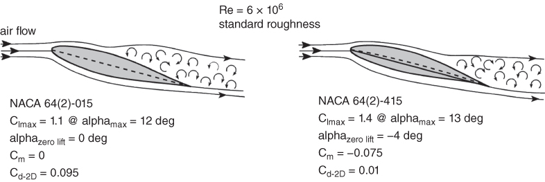
Figure 3.25 Camber effect comparison.
When compared with same aerofoil without camber (i.e. symmetric aerofoil), its introduction is necessary to delay separation with an increase in angle of attack, hence higher Clmax, at the cost of some drag and moment rise. Figure 3.25 shows that NACA 64(2) 415 with camber offers higher Clmax associated with higher αmax and negative zero lift angle at the expense of higher drag and nose‐down moment. A compromise is sought aiming to get the optimum camber that gives the maximum (L/D) with the least amount of associate Cm.
Figure 3.26 explains the physics by comparing test data at Re = 6 × 10⁶ of three aerofoil (NACA 652‐015, NACA 652‐015 and NACA 652‐415), one symmetric and the other two with camber.
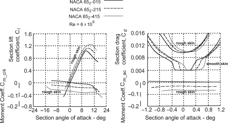
Figure 3.26 Comparing three test aerofoils (NACA 652‐015, NACA 652‐215 and NACA 652‐415).
Increase of camber shifts the lift graph to the left (Clα = 0 more negative), that is, increases sectional lift coefficient, Cl at the same α at the expense of increased drag and moment coefficients.
The amount of camber is linked with the thickness to chord level and its distribution. Typically, the camber is 2–8% for subsonic applications and 0–2% for supersonic applications. The lower the aircraft design speed, the more the camber may be.
There are special aerofoils suited to horizontal tailless aircraft such as all wing (blended‐wing body, BWB) aircraft. These wings have mixed camber, positive in the front and a small amount of negative camber at the TE to balance. These are known as camber with reflex. The NACA 23112 aerofoil (Figure 3.9) has small amount of reflex.
Figure 3.27 studies the NACA four‐digit aerofoil camber (NACA 1412, 2412 and 4412) and thickness (NACA 2412, 2415 and 2418) effects.

Figure 3.27 Comparing NACA four‐digit aerofoils (NACA 1412, 2412, 2415, 2418 and 4412),
The lift characteristics degrades after certain increase in thickness, in this case past a 15% thickness to chord (t/c) ratio. Since structural engineers prefer thicker aerofoils to attain structural integrity and increased wing internal volume for fuel accommodation, typically, for subsonic aircraft applications, the selection remains between 10 and 18% t/c. For low‐speed aircraft below Mach 0.3 the aerofoil thickness is on the high side; many successful aircraft have 15–18% t/c. But for aircraft operating above Mach 0.7, aerofoil thickness will depend on the wing sweep. Higher speed application with less wing sweep has lower t/c (see Figure 4.23 – Section 4.11).
Figure 3.28 shows typical trends in thickness and camber variations comparing NACA six‐digit aerofoil. Such trends also show in other NACA series aerofoil. The exact value must be read from the test data given in [6]. The camber effect of the other NACA series confirms similar characteristics as in the NACA six series shown in Figure 3.28 except that the NACA four‐digit does not have a drag bucket. The thickness effect shows practically no change in moment characteristics. Thickness effect can be seen as thicker the aerofoil more is the pressure drag on account higher blockage are and of small increase in contour length increasing the skin friction drag (at the same CL). However, thicker aerofoils offer benefits with better structural integrity, lower weight and increased volume that can accommodate more fuel, if required.
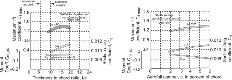
Figure 3.28 Typical trends in thickness and camber effects – comparing NACA six‐digit aerofoils.
Current research is being conducted on aerofoils with a self‐adaptive camber using smart materials to suit the full range of operational flight speed for the best L/D. Smart materials can be customised to generate a specific response to a combination of inputs. These materials include piezo‐electrics and electrostrictives, as well as shape memory alloy (SMA), which is lightweight and produces high force and large deflection.
3.9.2 Comparison of Three NACA Aerofoils
The NACA 4412, NACA 23015 and NACA 642‐415 are three commonly used aerofoils – there are many different types of aircraft that use one of these. Figure 3.29 compares these three popular NACA aerofoils (source NACA) to examine what is needed to make the choice.
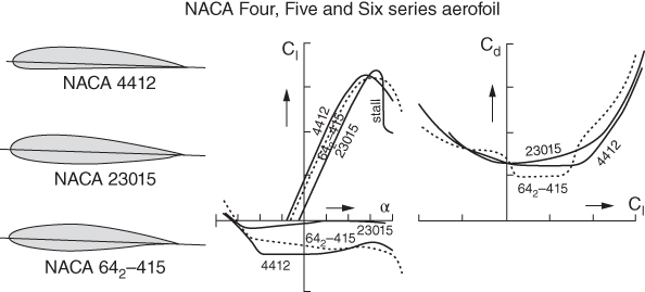
Figure 3.29 Comparison of three NACA aerofoils [6].
The NACA 23015 has sharp stalling characteristics; however, it can give a higher sectional lift, Cl and lower sectional moment, Cm, than others. Drag‐wise, the NACA 642‐415 has a bucket to give the lowest sectional drag. The NACA 4412 is the oldest and, for its time, was the favourite. Of these three examples, the NACA 642‐415 is the best for gentle stall characteristics and low sectional drag, offsetting the small drag due to the relatively not so high moment coefficient.
The five‐digit NACA 23015 gives the highest Clmax at higher angle of attack, α, but has abrupt stall not suitable for the ab initio club trainer but serves the utility category of aircraft. The benefits of the newer six‐digit NACA 642‐415 offers all round benefits with gentler stall characteristics including a lower Cm and a drag bucket to offer lower drag at low CL compared to four‐digit NACA 4414. However, the four‐digit NACA series is tolerant to production variation, hence it is popular in small aircraft designs as it is cheaper to manufacture.
The advanced NACA six‐digit series aerofoil came after NACA five‐digit series aerofoil making this successful aerofoil to fall behind.
An aerofoil designer must produce a suitable aerofoil that encompasses the best of all five qualities – a difficult compromise to make. Flaps are also an integral part of the design. Flap deflection effectively increases the aerofoil camber to generate more lift. Therefore, a designer also must examine all five qualities at all possible flap and slat deflections.
3.10 Centre of Pressure and Aerodynamic Centre
As stated earlier, an aerofoil is 2D bread‐slice like wing section is considered weightless. The pressure field around aerofoil develops forces and moment.
The centre of pressure, c.p., is defined as a point where moment vanishes and the resultant force of the pressure field acts. In other words, c.p. is the point where the resultant force represents the equivalent of what the pressure field generates on the aerofoil; the resultant force vector acting at the centre of pressure is the value of the integrated pressure field where there is no moment. The resultant force is resolved into lift and drag. Since the pressure field changes with angle of attack, the position c.p. changes accordingly. This makes c.p. a difficult parameter to deal with.
As the angle of attack, α, is increased, the aerofoil gets front loaded and the c.p. moves forward. With decrease of α the c.p. moves back. When α is reduced to a low value, for cambered aerofoil the inherent nose‐down moment may move the c.p. rearward outside of the aerofoil. Low resultant force at low angle of attack requires a large moment arm to balance, pushing the c.p. further aft. At zero lift, the c.p. approaches infinity. For a typical aerofoil, the c.p. stays within the aerofoil for the operating range. Figure 3.30 depicts the movement of centre of pressure, c.p., with a change in lift. The figure shows that, past αmax, the Cl drops rapidly – if not drastically – when stall is reached. Stalling starts at reaching αmax. It will be shown in Section 3.10.1 that c.p. is always aft of the quarter chord. This makes for a realistic aerofoil, as the aft is loaded with a nose‐down (−ve) moment. The extent of aft loading depends on how far behind is the minimum c.p. point. The second digit of the NACA six series gives the minimum c.p. point in tenth of the chord from the LE.
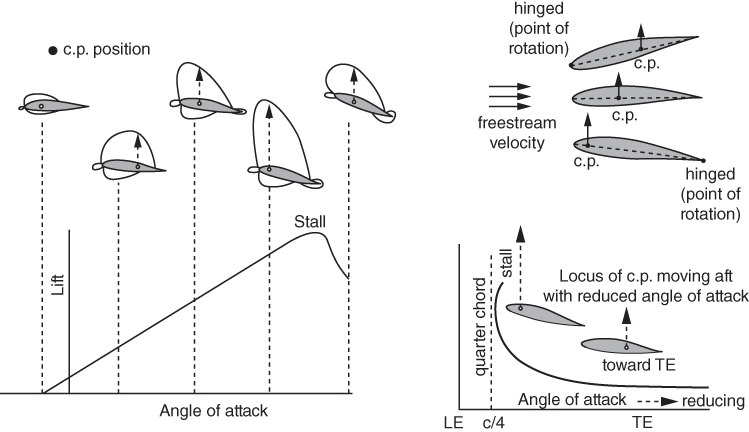
Figure 3.30 Movement of centre of pressure with change in lift.
The aerodynamic centre, ac, is concerned with moments about a point, typically on the chord line (Figures 3.31). It does not deal with force by itself. However, it is noticed that the moment about the quarter chord of the aerofoil is invariant to the angle of attack (dCm/dα = 0) until stall occurs. This point is invariant to α change and is known as the a.c., which is a natural reference point through which all forces and moments are defined to act. The ‘a.c.’ is close to the quarter chord point. There could be minor variations of the position of the a.c. around the quarter chord among aerofoils. To standardise, the fixed point at the quarter chord from the LE is also measured. In term of coefficient, these are Cm_ac and Cm1/4 are measured in wind tunnel tests. A symmetric aerofoil has Cm_ac = 0 but there is small variation of Cm1/4 with α variation. The relation between Cm_ac and Cm1/4 can expressed in mathematical relations as dealt with in Section 3.11.1. Aerofoil characteristics given in Appendix F show gives both the Cm_ac and the Cm1/4.

Figure 3.31 Aerodynamic centre invariant near the quarter chord (fractional chord position about which the moment is taken).
The a.c. offers much useful information. At the a.c., although the dCm/dα = 0, it has some moment (except symmetrical aerofoil) and is not the c.p., which is always aft of the a.c. The a.c. is an useful parameter in stability analyses when aircraft CG has to be taken into account. The higher the positive camber, the more lift is generated for a given angle of attack; however, this leads to a greater nose‐down moment. To counter this nose‐down moment, conventional aircraft have a horizontal tail with the negative camber supported by an elevator. For tailless aircraft (e.g. delta wing designs in which the horizontal tail merges with wing), the TE is given a negative camber as a ‘reflex’. This balancing is known as trimming and it is associated with the type of drag known as trim drag. Aerofoil selection is then a compromise between having good lift characteristics and a low moment.
When series of aerofoil are stacked up side by side to form a wing that is to be integrated with the aircraft, then contribution of isolated wing weight has to be considered its moment characteristics. Typically, wing Mean Aerodynamic Chord (MAC) (Section 4.8) represents its reference geometry to compute wing aerodynamic characteristics. The point of CG location is about which the wing moment is considered. The CG can be ahead or aft of the quarter chord point of the wing MAC. Chapter 18 explains that static stability requires to simultaneously satisfy (i) that aerofoil Cm has to be positive at α = 0 and (ii) dCm/dα has to be negative as well. A typical cambered aerofoil has a negative Cm at α = 0. Therefore, the wing will require an additional surface behind it (a small wing like horizontal tail at aft fuselage or a reflex wing TE) to keep nose up to retain static stability. The wing and empennage are dealt with in Chapters 4 and 6, respectively.
3.10.1 Relation Between Centre of Pressure and Aerodynamic Centre
Typically, the a.c. is within 22–27% of the aerofoil chord from the LE. Since the point varies from aerofoil to aerofoil, therefore, for standardisation, test results are given about a fixed point of quarter chord, c/4, from the LE. From the test result of a aerofoil moment around the quarter chord, the aerodynamic centre can be accurately determined and also given in a graph (Appendix F).
Figure 3.31 shows a typical aerofoil (NACA six series) with quarter chord c/4 and the aerodynamic centre, a.c., shown at a distance xc/4 and xa.c. from the LE, respectively. At the xc/4, the sectional lift, L, and moment Mc/4 are shown in the diagram (drag is small and its moment contribution is negligibly small).
3.10.1.1 Estimating the Position of the Aerodynamic Centre, a.c.
As mentioned before, the quarter chord xc/4 is at a fixed position and test results of Cm_c/4 are available [6]. Also, Cm_ac is invariant with respect to angle of attack, α (i.e. Cl). Taking the moment about the a.c. the moment equilibrium gives (moment contribution by drag is small as the moment arm is negligible). The aerofoil is considered weightless and the definitions of the aerodynamic coefficients are given in Equation (1.2).
Differentiating with respect to angle of attack α, it becomes (note that Cm_ac is constant),
where, m0 = slope of the CM_c/4 curve and a0 = is the lift curve slope.

m0 and a0 can be evaluated from the test results (Appendix F).
3.10.1.2 Estimating the Position of the Centre of Pressure, c.p.
Estimating c.p. is lot more difficult as it moves (Figure 3.30), with the operating range from mid‐chord, c/2, to a.c. at aircraft stall.
Let the aerofoil section lift l act at the aerofoil c.p. Taking moment about the quarter chord, c/4.
In coefficient form, Cl × (xc.p. – xc/4). + Cm_c/4 = 0
Substituting the value of Cm_c/4 from Equation 3.17 into this equation
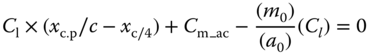
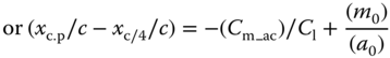
Cm_ac is negative for conventional aerofoil, that makes xc.p/c > xc/4, always.
Replacing m0/a0 = (xa.c./c – xc/4/c) from the relation given below Equation 3.16 in this equation it becomes:
It can be seen that the c.p. is aft of the a.c. At the a.c., although the dCm/dα = 0, it has some moment (except symmetrical aerofoil).
The centre of pressure and aerodynamic centre can be analytically determined if the aerofoil properties can be analytically expressed. Within in the operating range, the aerofoil lift characteristics can be expressed as a straight line and the moment characteristic is not exactly a straight line but can be tolerated as straight line; however the drag characteristics may not be amenable to fit as an equation of parabola resulting in inaccuracies. To obtain industry standard results, it is recommended that test data may be used [6].
It is stressed that the readers must understand the role of a.c. and c.p. This gives a good insight into how an aerofoil behaves.
3.11 Types of Stall
Section 3.3 describes the physics of stall phenomena over an aerofoil. It is essential that designers understand stalling characteristics because wing stall is an undesirable state for an aircraft to enter. Figure 3.32 shows the general types of stall that can occur. This section describes how these different types of stall affect aircraft design.
Figure 3.32 Stall pattern.
3.11.1 Gradual Stall
This is a desirable pattern and occurs when separation is initiated at the TE of the aerofoil; the remainder maintains the pressure differential. As the separation moves slowly towards the LE, the aircraft approaches stall gradually, giving the pilot enough time to take corrective action. The forgiving and gentle nature of this stall is ideal for an ab initio trainee pilot. The type of aerofoil that experiences this type of stall has a generously rounded LE, providing smooth flow negotiation but not necessarily other desirable performance characteristics.
3.11.2 Abrupt Stall
This type of stall invariably starts with separation at the LE, initially as a small bubble. Then, the bubble either progresses downstream or bursts quickly and catastrophically (i.e. abruptly). Aerofoils with a sharper LE, such as those found on higher‐performance aircraft, tend to exhibit this type of behaviour. At stall, Cm degrades to a sudden increase of nose‐down moment. Aircraft stall is affected by wing stall, which depends on aerofoil characteristics. Stall characteristics with high‐lift devices deployed have to be examined at the takeoff and landing operations. Thin aerofoil have abrupt stall. Aircraft with thin aerofoil are flown by experienced pilots trained to recognise the incipient stages of stall to take corrective actions in time.
A thin aerofoil with a sharp LE exhibits an abrupt stall.
3.12 High‐Lift Devices
For pilot ease and safety, takeoff and landing are done at the lowest achievable speed as conceived by the specification requirements. A large commercial transport aircraft cruising at about 500 kn at 39 000 ft altitude, lifts off at about 150 kn and approaches to land at about 130 kn. Flying less than a third of cruise speed is at high CL will require some sort of lift augmentation by incorporating some form of high‐lift devices that changes the aerofoil configuration from its retracted position (loosely termed ‘clean’) to a more cambered and extended chord aerofoil (loosely termed a ‘dirty’ configuration).
High‐lift devices are small aerofoil‐like elements that are fitted at the TE of the wing as a flap and/or at the LE. A typical high performance high‐lift device is shown in Figures 3.33. It is a double slotted Fowler flap with a slot at the LE of the wing. In this example, the Fowler flap system has a ‘vane’ to give the first gap for the slot followed by a flap that creates the gap for the second slot.
In typical cruise conditions, the flaps and slats are retracted within the contour of the aerofoil. Flaps and slats can be used independently or in combination. At low speed, they are deflected, rendering the aerofoil more curved as if it had more camber. The Fowler flap extends the chord, which increases the wing area. A typical flow field around the flaps and slats is shown in Figure 3.33. The entrainment effect through the gap between the wing and the flap allows mixing of boundary layer flow to remain attached in order to provide the best possible lift. Gaps and overlaps are to be optimised to obtain the best high‐lift.

Figure 3.33 High‐lift device.
In order to augment lift to achieve low‐speed capabilities, the deployment of high‐lift devices penalise by increase in drag and nose‐down moment, as well as the stall margin gets reduced associated with unfavourable abrupt stall. While it achieves the goal of lift‐off at shorter field length at takeoff, the drag increase degrades the climb rate and may prove critical to clear obstacles and changes the pitch attitude requiring high degree of trim to ease stick force. Approach to land occurs at steeper angles. These aspects are dealt with in detail in subsequent chapters.
In order to augment lift to achieve low‐speed capabilities, the deployment of high‐lift devices penalise by increase in drag and nose‐down moment, as well as the stall margin gets reduced and have unfavourable abrupt stall. While it achieves the goal of lift‐off at shorter field length at takeoff, the drag increase degrades the climb rate and prove critical to clear obstacles and changes the pitch attitude requiring high degree of trim to ease stick force. Approach to land occurs at steeper angles. These aspects are dealt with in detail in subsequent chapters.
A qualitative lift augmentation by using high‐lift devices is shown in Figure 3.34. While the lift curve slope dCl/dα is not greatly affected, the deployment of flaps gives a higher Cl at the same angle of attack, α, on account of an increased camber. Note that LE slot itself does change the camber holding on to the same α at zero lift, αCl = 0, but all other high‐lift devices reconfigure the basic aerofoil to a higher camber when αCl = 0 takes a more negative value.
Figure 3.34 Flap and slat lift characteristics.
There are various kind of high‐lift devices as shown in Figure 3.35, the choice depends on the category of aircraft as listed in Section 4.15. LE and TE devices are shown separately. A high‐lift system selectively combines as required for the design. Section 4.13 continues with high‐lift design and this is discussed in detail there.
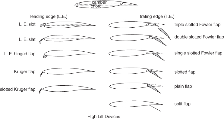
Figure 3.35 High‐lift devices.
Figure 3.36 lists the experimental values of the lift coefficients of aerofoil (lift augmentation by blown flaps is not dealt with here) at the landing configuration. These values are representative of types of NACA aerofoils and may be used if actual data are not available. When high‐lift devices are installed on a wing, its finite span 3D effects reduces the Clmax to a lower value of CLmax, as shown in Figure 4.31. This topic extends to wing flap design in Section 4.13.
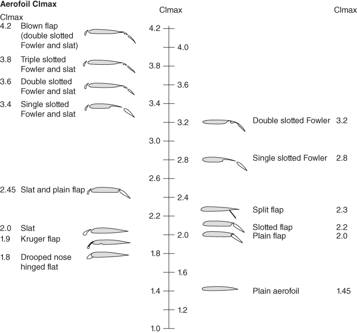
Figure 3.36 High‐lift devices and typical values of 2D Clmax.
Higher‐performance, high‐lift devices are complex in construction and therefore heavier and more expensive. Selection of the type is based on cost‐versus performance trade‐off studies – in practice, past experience is helpful in making selections.
Figure 3.37 depicts the corresponding distribution of the pressure coefficient Cp at an angle of attack of 15°.

Figure 3.37 Aerofoil Cp distribution characteristics.
Deflection of either the control surface or a change in the angle of attack will alter the pressure distribution. The positive y‐direction has a negative pressure on the upper surface. The area between the graphs of the upper and lower surface Cp distribution is the lift generated for the unit span of this aerofoil.
3.13 Flow Regimes
Disturbance in air creates pressure wave and if within the audible frequency range then it manifests as a sound wave. In other words, disturbance created by a moving object (a body, say an aircraft) travels through air at the speed of sound. As the speed of the object increases, the difference between the object speed and speed of sound decreases. Figure 3.38 shows the various flow regimes over an aerofoil (2D) section.

Figure 3.38 Flow regimes.
Approaching Mach 0.5, air molecules between the source and the limiting speed of sound start to coalesce and the effect is felt as compressibility effects offering some resistance to the moving object and is termed wave drag. Airflow over a curved surface accelerates higher than free stream velocity known as super velocity. Section 3.13.2 explains the compressibility effect on an aerofoil resulting from the onset of sonic flow at a point on account of the thickness distribution along the chord. The onset of wave drag is taken as a critical Mach number, Mcrit. Below Mach 0.5, the compressibility effects are weak and can be ignored. The body speed approaching around Mach 0.75, an arbitrary limit is imposed accepting a 20 count (ΔCD = 0.002) drag rise at the speed known as the drag divergence Mach number, MDD. Between MDD and speed of sound, the compressibility effect is strong with a complex mix of subsonic and supersonic flow regimes over the body as transonic flow. Also, the local coalescing of pressure appears as a local shock wave on the surface, which interacts with the local boundary layer with the potential to rupture the flow and to separate leading to the undesirable result of loss of lift.
To repeat, drag divergence is a sudden increase in drag. A 20‐count drag rise (CD = 0.002) at the Mach number is known as the drag divergence Mach (MDD), shown in Figure 3.38. The critical Mach (Mcrit) is the onset of the transonic flow field and is lower than the MDD. In the past, the NACA six‐digit series of aerofoils were used in aircraft flying at transonic speeds at relatively low MDD. Special attention is necessary when generating the aerofoil section designs that have a flat upper surface.
There several other ways to define drag divergence Mach. Airbus and Boeing take Mcrit when drag rises to ΔCD = 0.002 due to local shock forming on the wing at a critical point when transonic effects need to be considered. The onset of local shock formation is yet to reach a critical point as the highest Mach number for aircraft to cruise is the MCR when the compressibility effects are small enough to be ignored. The Douglas Aircraft Company (since taken over by Boeing) had another definition: when the rate of change of parasite drag, CDP with respect to aircraft Mach number, M, shows a 10% gain, that is, d(CDP)/dM = 0.1. These are arbitrarily accepted. It appears that civil aircraft design prefers ΔCD = 0.002 and military aircraft design prefers d(CDP)/dM = 0.1 to define the MDD. In this book, henceforth, the Boeing definition will be used based on the first author's work experience at the Boeing Aircraft Company, that is MCR and Mcrit and instead of Mcrit and MDD, respectively (Figure 3.38).
When the body speed reaches the speed of sound (Mach = 1), the pressure wave coalesces to a wave front known as a shock wave, it starts as normal shock ahead of the body with some thickness and subsonic flow behind the normal shock. As the body speed increases above that of sound, the shock wave gradually turns to oblique shock and gets attached to the body if it has a sharp edge. In 3D, the oblique shock is in the shape of a cone/wedge whose subtended angle reduces with increase in the body speed. Since the disturbance created by the body cannot travel faster than speed of sound, the flow field ahead of the shock cone/wedge remains undisturbed and is seen as a zone of silence.
This section is meant to give an overview of the physics for the readers to review and apply. Wing MDD and Mcrit are dealt in Section 4.11.
3.13.1 Compressibility Correction
Compressibility effects require application of correction factors (Prandtl–Glauert Rule); high‐subsonic and supersonic corrections differ slightly. In the following are some of the corrections of interest.
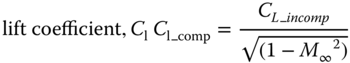
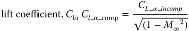
For low subsonic speeds below ≈0.3 Mach, the correction factors are small and can be neglected. For high‐subsonic speeds, the correction factor can be applied up to the onset of drag rise (Mcr, Boeing definition) ≈ 0.7 Mach as above this speed close to M∞ = 1.0, the correction diverges to unrealistic values. The same is true for the supersonic speed, the correction factor is applicable above Mach 1.3. Fortunately, supersonic aircraft flying below 1.4 Mach do not offer aerodynamic and economic gains.
In a way, theoretical analyses of supersonic flow is simple compared to incompressible flow analyses. For a low aspect ratio (AR) wing, further correction is required to obtain a lift curve slope. This book uses experimental data and the Prandtl–Glauert correction factor is not used.
3.13.2 Transonic Effects
This section explains the transonic effects resulting from the thickness distribution along an aerofoil chord. At high‐subsonic speeds, the local velocity along a curved surface (e.g. on aerofoil surface) can exceed the speed of sound, whereas flow over the rest of the surface stays subsonic. In this case, the aerofoil is said to be in transonic flow. At higher angles of attack, transonic effects can appear at lower flight speeds. Aerofoil‐thickness distribution along the chord length is the parameter that affects the induction of transonic flow. A local shock on account of supersonic flow interacting with the boundary layer can trigger early separation, resulting in unsteady vibration.
Transonic characteristics exhibit an increase in wave drag on account of the compressibility effect. There is a rapid drag increase. Military aircraft in hard manoeuvre can enter into such an undesirable situation, even at a lower speed. As much as possible, designers try to avoid, delay or minimise the onset of flow separation over the wing due to local shocks. These effects are undesirable but unavoidable; however, aircraft designers keep the transonic effect as low as possible.
The patented Whitcomb aerofoil section appeared later with a flatter top that delayed the Mcrit (Airbus/Boeing definition) to a higher Mach number. This was called the supercritical aerofoil section. It allowed the aircraft to fly faster with a 20 count wave drag rise. The geometrical characteristics exhibit a round LE, followed by a flat upper surface and rear‐loading with camber; the lower surface at the TE shows the cusp. All modern high‐subsonic aircraft have the supercritical aerofoil section characteristics. Figures 3.39 and 3.40 compare a typical transonic aerofoil (i.e. the Whitcomb section) and its characteristics with a NACA six series aerofoil. Manufacturers develop their own section or use any data available to them.
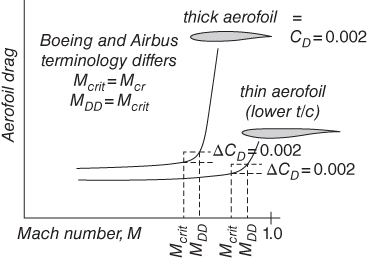
Figure 3.39 Wing sweep versus aerofoil thickness to chord ratio.

Figure 3.40 Transonic flow comparison (supercritical Whitcomb aerofoil).
Structural engineers prefer aerofoil sections to be as thick as possible, which favours structural integrity at lower weights and allows the storage of more fuel onboard. However, aerodynamicists prefer the aerofoil to be as thin as possible to minimise the transonic flow regime in order to keep the wave drag rise lower. Wing planform shape influences the choice of aerofoil thickness. Wing planform is dealt with in Chapter 4.
The choice decides the extent of wing sweep required to lower the t/c ratio to achieve the desired result (i.e. to minimise the compressible drag increase for the cruise Mach number) while also satisfying the structural requirements. To standardise drag rise characteristics, the flow behaviour is considered to be nearly incompressible up to Mcr and can tolerate up to Mcrit, allowing a 20‐count drag increase (ΔCD = 0.002).
3.13.3 Supersonic Effects
As a result of the presence of shock wave, the flow physics of supersonic flow differs from subsonic flow. In case of supersonic flow, the disturbance generated by the body cannot travel ahead of the body and stays within the shock cone. Subsonic disturbances travels ahead of the object at the speed of sound.
Figure 3.41 shows the shock pattern over the three well‐used types of supersonic aerofoil of six supersonic aerofoils in Figure 3.16.
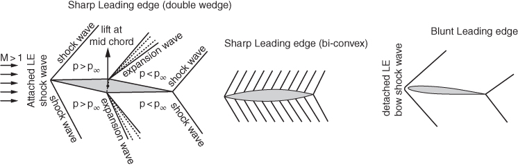
Figure 3.41 Shock patterns over three types of supersonic aerofoil.
The double wedge aerofoil has a sharp LE and the oblique shocks stay attached. Reaching a point of inflection, expansion waves develop to negotiate the favourable pressure gradient to accelerate flow reaching the TE again in a shock wave.
The biconvex aerofoil also has sharp LE but on smooth curvature the oblique shocks are distributed until the inflection is from where the distributed expansion continues with flow accelerating ending in tail oblique shock.
The blunt LE thin aerofoil has a small normal shock with a small zone of subsonic flow. As the aerofoil slope changes rapidly, the shock turns to oblique shock with an angle corresponding to the free stream Mach number (Figures 3.40 and 3.41). Downstream, the shock pattern is like this too. The NACA 66 206 is an example of this kind. Due to manufacturing limitation and operational maintenance, a blunt LE with a very small LE radius is widely used, especially if the wing is within the shock cone (see Section 4.13).
A thin supersonic aerofoil with a sharp LE in fully immersed supersonic flow gives (linear thin aerofoil theory) the following.

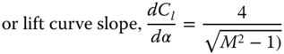
Supersonic aerofoils are very thin (4–% t/c) and have little camber. The cruise CL values are low, that is, it operates at low α. These conditions allow the governing nonlinear equations to be linearised, yielding good results within the operating range. To obtain pressure distribution around the aerofoil, the linearised supersonic equations can then be split into three components of: (i) straight line at an angle of attack, α, (ii) aerofoil camber at zero angle of attack and (iii) thickness distribution of the aerofoil as shown in Figure 3.42 and superimpose the solutions by adding to get the results.

Figure 3.42 Flow over a supersonic aerofoil.
The low thickness to chord ratio (t/c), low camber and low angle of attack, α, indicate that the shock wave is very weak and its angle, β, can be approximated to a Mach wave angle, μ (i.e. β ≈ μ, refer to Section 3.3). This simplifies the wing design considerations discussed in Section 4.13.
3.14 Summary
Aerofoil design is a subject on its own involving theoretical CFD and extensive wind tunnel tests beyond the scope of this book. Since the 1980s, with the advent of CFD, the approach to aerofoil design started changing. As CFD capabilities became more refined, it is now possible to producing credible 2D aerofoil characteristics (lift, drag, moment and stall characteristics) in high fidelity, minimising wind tunnel testing to the point of making it nearly redundant, saving cost and time. CFD is now accepted as a digital wind tunnel to obtain aerofoil characteristics. This book only deals with the NACA series aerofoil. It is recommended to use aerofoil test data [6]. Six sets of suitable aerofoil experimental data are provided in Appendix F. This section gives a coarse guide to making an aerofoil selection.
This chapter covers a considerable amount of information, many in graphic representations to facilitate the newly initiated to appreciate the underlying technologies in choosing an aerofoil. The heart of aircraft design is in the selection of an appropriate aerofoil to arrive at the wing planform geometry fit for the purpose, that is, mainly to offer high‐lift/drag ratio (L/D), low drag and low moment for the wing. The primary parameters of interest in selecting aerofoils are Clmax, Clα, αstall, αCl = 0, Cm‐ac and Cdmin. There could be several candidate aerofoils with similarities in characteristics to satisfy performance requirements. It is also important to consider how tolerant the aerofoil is to manufacturing deviation. It requires experience to select an aerofoil relying on past experience and currently operating aircraft performances.
It is stressed here that aerofoil selection is not a standalone exercise. The degradation of aerodynamic properties of a 2D aerofoil as finite wing sections (see Section 4.7) has to be considered at this stage. Also the Clmax, αstall, αzero‐lift, Cm‐ac and Cdmin characteristics of high‐lift devices deployed, as well stall characteristics, need to be examined in choosing a suitable aerofoil.
The compressibility effect of airflow influences the shaping of aircraft. Airflow below Mach 0.3 behaves as nearly incompressible – in such a regime all aircraft are propeller (piston engine) driven. From Mach 0.3 to 0.6 compressibility effects gradually build up but propellers are still effective up to Mach 0.6, however, its magnitude is small enough to be ignored. Above Mach 0.6, aircraft component geometry has to cater for compressibility effects. Jet propulsion becomes more suitable above Mach 0.6. Therefore, the aircraft component configuration is divided in two classes, one suited to flying below Mach 0.6 and one above Mach 0.6. The latest propeller technology is pushing flight speed towards Mach 0.7.
Aerofoil selection is mission specific. Aircraft speed requirements influence the aerofoil choice, of course, the other considerations, for example low Cm, low Cd, high t/c and so on, in a best compromise have to be taken into account. Based on the specified aircraft design speed, aircraft are grouped in the following category. This gives the Re of the wing.
Low subsonic (below Mach 0.5) – propeller driven – (Λ1/4 wing sweep ≈0 ± 5% degree)
Gliders/Microlights operating around 80 mph in a very low Re No. Typical suitable aerofoils are chosen from the NACA four‐digit, Liebeck, Lissaman, Eppler aerofoils series. Some of these offer laminar flow characteristics. Typical (t/c) ratio is around 0.14–0.18. This class of aircraft is not dealt with in this book.
Home‐builds (Light Sports Aircraft – LSA) operating at around 120 mph with a low Re. A well proven NACA four‐digit serves well. The LSA certification category of aircraft is not dealt with in this book. The design approach for this class is similar to the club trainer/recreational category of aircraft given next. Typical (t/c) ratio is around 0.12–0.18.
Club trainers/recreational aircraft (Normal Category, FAR 23) operating at around 150 mph in a low Re. Ab initio trainer aircraft must have gentle and gradual stall characteristics and be of a forgiving type, providing safety. Typical suitable aerofoils for trainer aircraft are chosen from the NACA four‐digit series. The NACA five‐digit series may be considered for recreational aircraft. With abrupt stalling characteristics, the NACA five‐digit series are not suitable for trainer aircraft. Of late, the GAW aerofoils have been used in this category of aircraft. Typical (t/c) ratio is around 0.12–0.18.
Aerobatic Category (FAR 23) operating around 200 mph. On account of requiring better performance and handling qualities during inverted flying, a symmetrical aerofoil may also be considered. The NACA four‐ and six‐digit aerofoils suit well. Typical (t/c) ratio is around 0.12–0.16.
Utility/Regional aircraft operating around 300 mph. This class of aircraft are flown by experienced pilots in fare‐earning sorties at higher speeds but are well below compressibility effects to be considered. NACA five‐ and NACA six‐digit aerofoils are now more commonly used.
High‐subsonic (Mach 0.7 to Mach 0.95) – jet propulsion – (Λ1/4 wing sweep ≈10–35°)
Incorporating wing sweep influences the choice for aerofoil t/c as shown in Figure 4.27 (forward sweep aircraft are uncommon but possible). In general, in this category of aircraft design, industries develop their own aerofoils and these are kept ‘commercial in confidence’.
The Bizjet/regional jet operating between Mach 0.7 and 0.85 requires a swept wing. The use of the NACA six‐digit aerofoil dominates high‐subsonic aircraft design. Thickness to chord ratio t/c is around 0.09–0.15, depending on sweep (see Section 4.11.2).
Commercial jets operating between Mach 0.75 and 0.92. Aircraft with longer range missions have higher speed requiring relative wing Λ1/4 sweep of 20–35° that influences the choice of aerofoil t/c. These high‐subsonic aircraft operating in transonic regimes require careful consideration. Industry accepts a wave drag rise (compressibility effect) of 20 counts (see Section 4.11.1) for high‐speed cruise at MDD. The higher the MDD, the thinner the t/c for the given wing sweep. The current practice is to adopt a supercritical aerofoil. Supercritical aerofoils have a good stretch of laminar flow from the LE. Laminar flow characteristics are sought after, but the extent of laminar flow during operation is not guaranteed on account of natural surface degradation during usage. There are excellent supercritical aerofoils in the NASA SC series. Six‐digit aerofoils have also been used. The t/c values are around 0.12–0.15.
Supersonic category [Λ1/4 wing sweep ≈0–60° (delta wing)]
Combat aircraft operating between Mach 1.8 and 2.4. Concorde was the only commercial aircraft in operation; a new generation of supersonic aircraft is now under consideration. On account of the presence of shock waves, the supersonic aerofoil sections are of quite a different class for the reasons dealt with in Section 3.8.3.10. These are necessarily very thin aerofoils, typically with a t/c around 0.04–0.07.
Table 3.3 gives a few examples of NACA aerofoils that are widely used in industry. Note the absence of aerofoils used by Airbus and Boeing, as they develop their own.
| Conventional Aircraft: | Wing Root Aerofoil | Wing Tip Aerofoil |
| Propeller Driven Aircraft | ||
| Aero Commander 200 | NACA 23015 | NACA 4412 |
| Aero Commander 500 Shrike | NACA 23012 | NACA 23012 |
| Aeronca 11‐AC Chief | NACA 4412 | NACA 4412 |
| Auster J1B | NACA 23012 | NACA 23012 |
| Avro 748 | NACA 23018 | NACA 4412 |
| Beagle B.121 Bulldog | NACA 63‐615 | NACA 63‐615 |
| Beech 300 Super King Air | NACA 23018 | NACA 23012 |
| Beech 77 Skipper | NASA GA(W)‐1 | NASA GA(W)‐1 |
| Britten‐Norman BN‐2A Islander | NACA 23012 | NACA 23012 |
| Canadair CL‐215 | NACA 4417 mod | NACA 4417 mod |
| Cessna 150 | NACA 2412 | NACA 0012 |
| Cessna 170 | NACA 2412 | NACA 2412 |
| Shorts S312 Tucano T.Mk1 | NACA 63A415 | NACA 63A212 |
| RANS S‐16 Shekari | NASA GA(W)‐1 | NASA GA(W)‐1 |
| Supermarine 378 Spitfire IX | NACA 2213 | NACA 2209.4 |
| Shorts SC.7 Skyvan | NACA 63A414 | NACA 63A414 |
| Shorts SD‐330 (C‐23) | NACA 63A418 | NACA 63A414 |
| Shorts SD‐360 | NACA 63A418 | NACA 63A41 |
| SIAI‐Marchetti SF.600 | NASA GA(W)‐1 | NASA GA(W)‐1 |
| Jet Propulsion Aircraft | ||
| Cessna 560 Citation V Excel | NACA 23014 mod | NACA 23012 |
| Gulfstream Aerospace GIV | NACA 0012 Mod | NACA 64A008.5 Mod |
| Learjet 55 | NACA 64A109 | NACA 64A109 mod |
| Learjet 60 | NACA 64A109 mod | NACA 64A109 mod |
| Supersonic Combat Aircraft | ||
| Boeing F‐15 Eagle | NACA 64A006.6 | NACA 64A203 |
| Lockheed F‐104 | Biconvex 3.36% | Biconvex 3.36% |
| Lockheed Martin F‐16 | NACA 64A204 | NACA 64A204 |
| McDonnell Douglas F‐15 Eagle | NACA 64A006.6 | NACA 64A203 |
| McDonnell Douglas F‐18 Hornet | NACA 65A005 mod | NACA 65A003.5 mod |
| McDonnell Douglas F‐4 Phantom II | NACA 0006.4‐64 mod | NACA 0003‐64 mod |
| North American Aviation RA‐5C | NACA 65A005 | NACA 65A005 |
| Northrop F‐5 Tiger | NACA 65A004.8 | NACA 65A004 |
The trends in the relationship of various parameters are shown in Figures 3.22, 3.31, 3.22 and 3.33. These show the trends for readers to compare and establish what are the desirable characteristics for the aerofoil to be chosen. In short, these graphs indicate some important aerodynamic properties that are summarised next. Table 3.4 gives the qualitative lists on the advantages and the disadvantages of the NACA series aerofoil.
Table 3.4 Generalised summary (see Section 3.15 at the end of Chapter 4).
| Aerofoil | Desirable | Undesirable | Application |
| NACA four‐digit | good gentle stall | moderate Clmax | Low‐speed application |
| (Manufacturing deviation) | very tolerant | high Cm‐ac | ab initio trainer aircraft |
| Surface roughness | tolerant | high profile drag | small aircraft, club usage, empennage design |
| NACA five‐digit | high Clmax | abrupt stall | moderate speed |
| low Cm‐ac | high profile drag | utility aircraft | |
| (Manufacturing deviation) | intolerant | ||
| Surface roughness | tolerant | ||
| NACA six‐digit | acceptable stall | wide range of designs | |
| good Clmax | (all category, extending | ||
| moderate Cm‐ac | to high‐subsonic operation | ||
| low profile drag (drag bucket) | thin sections for supersonic designs) | ||
| (Manufacturing deviation) | somewhat tolerant | ||
| Surface roughness | intolerant | ||
| GAW aerofoil | very high Clmax | not many aircraft using it | |
| high αstall | |||
| z | low profile drag in cruise (drag bucket) | tin section to supersonic designs) | |
| (Manufacturing deviation) | somewhat tolerant | ||
| Surface roughness | intolerant | ||
| Supersonic aerofoil | These are different class of aerofoil with considerable low values of Clmax and αstall. | ||
| Post stall state shave Clmax extend to around 20°, allowing high α manoeuvres. With | |||
| additional vortex lift with wing strake, it can extend to as high as around 40° manoeuvres. | |||
Figure 3.43 gives some of the well‐used aerofoil parameters. Surface roughness reduces the Clmax and increases Cdmin from the smooth (clean) surface aerofoil data. Rough surfaces represent an operational environment. Suggestions given next are from well‐proven NACA aerofoils widely in use.

Figure 3.43 NACA series aerofoils.
Figure 3.43 shows that the five‐digit NACA 23015 gives the highest Clmax at a higher angle of attack, α, but has abrupt stall characteristics not suitable for the ab initio club trainer, however, it serves utility category aircraft. The benefits of the newer six‐digit NACA 642‐415 are that it offers all round gains with gentler stall characteristics, lower Cm and a drag bucket to offer lower drag at the design Cl. The four‐digit NACA series aerofoils are tolerant to production variation, hence they are popular in small aircraft designs being cheaper to manufacture.
Wing planform shape (dealt with in Chapter 4) influences the choice of aerofoil thickness as shown in Figure 4.20. The figure gives the relation between wing aerofoil t/c and aircraft design speed within the band of wing sweep. Increase of aircraft speed decreases aerofoil t/c.
3.14.1 Simplified Aerofoil Selection Methodology
A simplified step‐by‐step generalised approach to making an aerofoil selection from available test data (NACA/NASA series) is outlined in a generalised manner so as to give a feel for the process: in industry it is done in a more rigorous manner (this is not the only way to select an aerofoil). In most large aircraft manufacturing companies, there is a separate group of researchers who develop advanced technologies. The role of aircraft designer is to interact with the researchers to develop a suitable advanced aerofoil to perform better than the competition. Aerofoil design is now very mature; to get a better one is not easy. Similar classes of NACA/NASA aerofoils have characteristics close enough to serve many smaller aircraft.
Aerofoil selection must match the requirements of the wing capability, hence it is finalised along with the considerations of wing design as summarised in Section 4.19 to meet the mission specifications. In civil aircraft design, aerofoils with good L/D capability are sought. Aerofoils show best L/D at their design Cl. Test results have to be studied to obtain the design Cl for the NACA four‐ and five‐digit aerofoils. For combat aircraft, Cl has to cover a wider range catering for manoeuvres as well. The step‐by‐step approach is given next.
- Step 1
The first task is the find the design CL for the new aircraft project. For civil aircraft, this is where the aircraft operates for the longest time. In transport aircraft, this is at the mid‐cruise weight flying at a Long Range Cruise (LRC) Mach number.
Given here are some typical design CL values for some classes of aircraft (more details in Section 4.19). Higher wing loads (W/SW) give higher design CL, operating at same‐speed altitudes.
| Aircraft category | Aircraft design CL | Typical preferred aerofoila) |
| Large transport aircraft | ≈0.25–0.35 | NACA six‐digit |
| Regional jets/Bizjets | ≈0.3–0.4 | NACA five‐ and six‐digit aerofoil |
| Small club class aircraft | ≈0.3–0.4 | NACA four‐digit aerofoil |
| Jet trainer | ≈0.15–0.2 | NACA six‐digit aerofoil |
| Combat aircraft | ≈0.1–0.2 | Supersonic aerofoil |
These are only typical NACA type suggestions. There are many other kinds that can be considered.
- Step 2
Convert (see Section 4.9.4) the finite span wing design CL to a 2D aerofoil Cl. Given next are some 2D aerofoil design Cl values that may be used at this stage. These coarse factors depend on the wing AR. This is not an industrial practice; that is considerably more rigorous using CFD, but it can start until the CFD generated aerofoil design Cl value is available. Unless the aircraft configuration has some wing body blending, the contribution to lift by the rest of aircraft is less than 3% and can be neglected. Oswald's efficiency factor, e (Section 4.9.3), gives the suitable factor taking AR and other effects into account.
| Aircraft category | AR | Factor | Aerofoil design Cl | |
| Large transport aircraft | 6–8 | ≈0.8–0.85 | ≈0.3–0.4 | |
| Large transport aircraft | 8–10 | ≈0.9–0.95 | ≈0.3–0.45 | |
| Regional jets/Bizjets | 6–8 | ≈0.8–0.85 | ≈0.3–0.4 | |
| Small club class aircraft | 5–6 | ≈0.7–0.8 | ≈0.4–0.5 | |
| Jet trainer | 4–6 | ≈0.7–0.8 | ≈0.2–0.3 | |
| Combat aircraft | Case to case based study is required. A coarse way to initiate | |||
| combat aircraft study is to take the wing design CL as the aerofoil Cl | ||||
- Step 3
The higher the camber, the higher the Cl at the same angle of attack, α. It is a desirable property but Figure 3.27 shows that a higher camber gives a higher Cm‐ac, an undesirable property. Camber shifts the zero lift angle αCl = 0 and the Cd.
Lowest values of Cd and Cm‐ac are preferred but both at the lowest may not be possible. This requires seeking the extent of camber required that can compromise between Cd and Cm‐ac, the lower the better. The NACA four‐digit aerofoil camber is given by the first number (only camber extents 2 and 4% of chord length are considered). The NACA five‐digit aerofoil camber is also given by the first number (camber of 2% of chord length is considered) However, the NACA six‐digit series does not give the camber but the second digit indicates the location of minimum Cp: important information as an indication for Cd and Cm‐ac that requires examining the graphs. The second digit of a combat aircraft extends from 3 to 6.
- Step 4
Decide the aerofoil thickness to chord ratio, t/c. Structural engineers prefer a thicker t/c that gives better rigidity lowering wing weight and offers provision between the spars to accommodate bigger volume for fuel storage. On the other hand, aerodynamicists desire thinner aerofoils to keep drag, Cd, low. Wing sweep (Section 4.8) permits an increase in the t/c. Typically, low subsonic aerofoils have a t/c between 12 and 18% and high‐subsonic aerofoils have t/c between 9 and 15%. The thickness to chord ratio, t/c, may vary along the wing span, being lowest at the tip section. In the case of a supersonic aerofoil, t/c ≈ 0.05 and camber is nearly zero.
- Step 5
Lastly, high Clα is sought. Figure 3.43 indicates that most subsonic aerofoils have Clα around 0.105 ± 5% per degree. Interestingly, the choice of Clmax comes later. Ab initio trainers prefer high Clmax and high αstall.
- Step 6
Examine the aerofoil characteristics with a high‐lift device. The NACA test graphs give data with a split flap. Absence of full details of aerofoil characteristics with contemporary flaps restrict the study in this book.
Other import aspects are to examine is the post‐stall behaviour of the aerofoil with and without high‐lift devices and how tolerant the aerofoil characteristics will be under production variations. Ab initio trainers require gentle and gradual stall that offers safety.
Although operational usage cannot guarantee laminar flow, aerofoil selection with a good laminar flow characteristic is desirable.
Start with picking up several suitable aerofoil sections (say 3–5) that have the design Cl. Choose the higher t/c ratio permitted by the wing sweep for the category of aircraft as given before. Next, to plot and superimpose the characteristics to compare and make the final choice.
Aerofoil selection for the worked out examples of Bizjet, Advanced Jet Trainer (AJT) and Turboprop Trainer Aircraft (TPT) are carried out in Chapter 8.
Since no single aerofoil can offer all of the desired properties at its maximum, compromise is required.
3.15 Aerofoil Design and Manufacture
Aerofoil design and manufacture are very important processes in any new aircraft project. Success depends on the fidelity to adhere to accuracy so that it performs as predicted. These are involved topics for which special study/training is required and are beyond the scope of this book.
This section is meant to make newcomers aware of the situation and give what is expected, should they be interested in pursuing the subject for research or production. Aerofoil design is theory intensive and special courses are offered by all aeronautical institutes. There are two ways to design aerofoils:
- the direct aerofoil design method
- the inverse aerofoil design method
After obtaining the suitable aerofoil, the aircraft designers progress with the aircraft design (the objective of this book). The finished product is drawn and then passed on to the production engineers to be manufactured. The role of aircraft designer is to work in an integrated product and process development (IPPD) environment as part of a team, bridging all sides, to make the product right first time. The Chief Engineer must have a good grasp of all aspects of aircraft design to integrate various components as a system.
3.15.1 Direct Aerofoil Design Method
This method involves theoretical analyses of a given aerofoil geometry drawn from designers' past experiences and data banks. The analyses starts with the inviscid flow considerations that simpler to solve, which gives a good estimates of dCl/dα. For other parameters, for example, Clmax, Cm and so on, viscous flow considerations involved with nonlinear differential Navier–Stokes equations are to be analysed; these are hard to solve if not sometimes impossible. Basically, the analytical procedure deals with tackling the two influencing parameters, the camber‐line geometry and the thickness distribution along it, conducted at several angles of attack. In earlier days without computers, this was a time consuming process.
The results obtained from theoretical analyses necessitate substantiation by wind tunnel tests of several aerofoil geometries in a parameter manner to choose the best from the lot, not really an efficient way to optimise. The NACA four‐ and five‐digit family of aerofoils were developed in this way. This is a lengthy, difficult and expensive process that could give a better aerofoil but the researchers want to achieve more.
3.15.2 Inverse Aerofoil Design Method
To overcome the limitations faced by the direct method, researchers succeeded by attempting an inverse method to analyse. The process starts with establishing an achievable superior Cp distribution and then making complex theoretical analyses requiring solution of difficult equations to find the matching geometry, if required iterating the Cp distribution to bring out what is achievable close to the specified one. This process delivers better aerofoils and has delivered new aerofoil identification designations.
3.15.2.1 Current Practice
Numerical methods for solving differential equations have been prevailing for some time. Solving the Navier–Stokes equations in compressible viscous flow was difficult, if not impossible in certain situations. Mathematicians devised methods to discretise the difficult nonlinear partial differential equations into algebraic forms, which are solvable. During the early 1970s, CFD results of simple 2D bodies in inviscid flow were demonstrated showing that certain parameters were comparable with wind tunnel test results and analytical solutions.
With more refinement in the numerical algorithm and with progress in computer processing power, the aerofoil design process has changed. Today, optimised aerofoil geometry can be found at a fraction of cost and time compared to the older methods. The confidence in the accuracy of CFD results for 2D aerofoils reached points where wind‐tunnel tests for substantiation could be reduced to a few tests. The 2D aerofoil CFD results are now acceptable to the certification agencies. CFD analyses is now seen as a digital wind tunnel.
There are excellent free aerofoil design software packages developed by well‐known researchers/academics available in the market. Some of them are extensively used in industry, large or small.
3.15.2.2 Manufacture
Manufacturing an accurate wing profile with aerofoil shaped ribs was possibly harder than designing them. It was difficult to produce large components in exact dimensions with the desired low tolerance that incurred a large number of rejections. The production process requires specified tolerances; the aerodynamicists want them as low as possible and the production engineers want them as high as possible. The compromise will associate with a corresponding loss of quality resulting in drag rise, moment change and degradation in Clmax. The full‐scale drawing of large aerofoils (say in the order exceeding 10 ft) had to be marked around the technician sitting inside it with a multitude of heavy weight location pins, which not amenable to maintaining tight tolerance. The lofting of wing skin required trial and error methods with some wastage. It was a painful process. The manual riveting had dimples, there were mismatches at the joints, waviness in the wing skin and so on. These methods could not avoid some costly rejections of the finished components.
All changed with the adaptation to the computer‐aided engineering (CAE) (CFD/Finite Element Method (FEM)/CAD/CAM etc.) method; a computer‐based design and manufacturing process. Today, accurate CAD modelling/drawings have dispensed with manual lofting and tighter tolerances can be specified as the CAD files can be directly sent to microprocessor‐based Numerically Controlled (NC) machines that can machine/cut/rivet automatically at higher accuracy and at higher speeds that were hitherto impossible. The rejection rate has come down, man‐hours have come down and machine hours have reduced.
It is strongly recommended that the readers may compare the finished surfaces of some older aircraft designs, say the class of the Mustang P, Douglas DC3 and so on, with some newer aircraft designs, say the class of F35, Airbus 320 and so on, to get a feel for the difference.
3.16 Aircraft Centre of Gravity, Centre of Pressure and Neutral Point
So far, mainly aerofoil aerodynamics has been dealt with. Two important aircraft parameters: (i) the aircraft CG and (ii) the aircraft Neutral Point (NP), need to be defined and explained at this early stage as they will be used in subsequent chapters for the whole aircraft. Shaping and positioning of aircraft components, for example, wing planform, fuselage shape, nacelle/intake shapes and empennage are established by satisfying the position of aircraft CG with respect to the location of the aircraft NP.
3.16.1 Aircraft Centre of Gravity (CG)
CG is the point where the resultant weight of all the assembled aircraft components and equipment acts vertically downward. Aircraft CG has to be computed, shown in the worked‐out examples in Chapter 10. Assembling the aircraft components by placing them in relation to each other is to be made in a way that will keep the aircraft CG location in a desirable place. If requires, internal equipment can be repositioned to bring the CG to the desired location. Centre of pressure, c.p., and aerodynamic centre, a.c., are discussed in Section 3.11.1.
3.16.2 Aircraft Neutral Point
Aircraft NP (see Section 10.5) is associated with the location of the aircraft CG to assess aircraft stability. If aircraft CG is at the NP then the aircraft becomes neutrally stable, hence it is called the NP; the aircraft dM/dα = 0.
The differences between aircraft centre of pressure, wing aerodynamic centre and aircraft NP are summarised in Section 3.16.3.
3.16.3 Summary
- CG is the point where the resultant weight of all the assembled aircraft components and equipment acts vertically downward.
- Centre of pressure, c.p., of an aircraft is the point where the lift acts. It has nothing to do with the aircraft CG.
- Aerodynamic centre, a.c., is the point in the weightless aerofoil/wing where the pitching moments are invariant to the changes in angle of attack. It also has nothing to do with the aircraft CG.
- NP is a fixed point for the aircraft configuration and is associated with the location of aircraft CG, which can vary depending how the aircraft is loaded with payload and fuel. Aircraft CG located at the NP makes aircraft neutrally stable, hence the name.
References
- 1. Shapiro, A. (1953 and 1954). The Dynamics and Thermodynamics of Compressible Fluid Flow, vol. 1 and II. New York: Ronald (Wiley) Press.
- 2. Kuethe, A.M. and Chow, C.‐Y. (1986). Foundations of Aerodynamics. Wiley.
- 3. Bertin, J.J. and Cummings, R.M. (2009). Aerodynamics for Engineers. Prentice Hall: Pearson.
- 4. Anderson, J. (2011). Fundamentals of Aerodynamics SI. McGraw Hill.
- 5. Schlichting, H. and Gersten, H. (2003). Boundary Layer Theory, 8e.
- 6. Abbott, I.H. and von Doenhoff, A.E. (1949). Theory of Wing Sections, Including a Summary of Aerofoil Data. New York: McGraw Hill.
- 7. Kuchemann, D. (2012). The Aerodynamic Design of Aircraft. AIAA.
- 8. ESDU. Website. Available online at: www.esdu.com/cgi‐bin/ps.pl?sess=unlicensed_1180626100613ksk&t=gen&p=home (accessed June 2018).
- 9. Lednicer, D. Airfoils of US and Canadian Aircraft. Available online at: www.aerofiles.com/aerofoils.html (accessed June 2018).
- 10. Lednicer, D. (2010). The Incomplete Guide to Airfoil Usage. Available online at: http://m-selig.ae.illinois.edu/ads/aircraft.html (accessed June 2018).
- 11. USAF DATCOM. (2017) Public domain aeronautical software. Available online at /www.pdas.com/datcom.html (accessed June 2018).