
CHAPTER 12 Ellipse Detection
12.1 Introduction
As seen in the previous chapter, many manufactured goods are circular or else possess distinctive circular features. This consideration makes it imperative to have an efficient set of algorithms for detecting circular shapes in digital images. However, in many situations such objects are viewed obliquely, and so efficient ellipse detectors are also required. Furthermore, some objects are actually elliptical, which also provides motivation for finding effective ellipse detection algorithms.
This chapter describes some of the algorithms that have been developed for this purpose. We concentrate on parallel algorithms inasmuch as sequential methods have already been covered in Chapter 7. In addition, parallel algorithms such as the Hough transform tend to be more robust. In fact, all the algorithms described here are based on one or other form of the Hough transform. Although Duda and Hart (1972) considered curve detection, the first method that made use of edge orientation information to reduce the amount of computation was that of Tsuji and Matsumoto (1978). Their ingenious method is described in the next section.
12.2 The Diameter Bisection Method
The diameter bisection method of Tsuji and Matsumoto (1978) is very simple in concept. First, a list is compiled of all the edge points in the image. Then, the list is sorted to find those that are antiparallel, so that they can lie at opposite ends of ellipse diameters. Next, the positions of the center points of the connecting lines for all such pairs are taken as voting positions in parameter space (Fig. 12.1). As for circle location, the parameter space that is used for this purpose is congruent to image space. Finally, the positions of significant peaks in parameter space are located to identify possible ellipse centers.
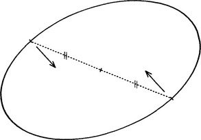
Figure 12.1 Principle of the diameter bisection method. A pair of points is located for which the edge orientations are antiparallel. If such a pair of points lies on an ellipse, the midpoint of the line joining the points will be situated at the center of the ellipse.
In an image containing many ellipses and other shapes, naturally there will be many pairs of antiparallel edge points, and for most of these the center points of the connecting lines will lead to nonuseful votes in parameter space. Such clutter of course leads to wasted computation. However, it is a principle of the Hough transform that votes must be accumulated in parameter space at all points that could in principle lead to correct object center location. It is left to the peak finder to find the voting positions that are most likely to correspond to object centers.
Not only does clutter lead to wasted computation, but the method itself is computationally expensive. This is because it examines all pairs of edge points, and there are many more such pairs than there are edge points (m edge points would lead to ![]() pairs of edge points). Indeed, since there are likely to be at least 1000 edge points in a typical 256 × 256 image, the computational problems can be formidable. The situation is examined more carefully in Section 12.6.
pairs of edge points). Indeed, since there are likely to be at least 1000 edge points in a typical 256 × 256 image, the computational problems can be formidable. The situation is examined more carefully in Section 12.6.
The basic method is not particularly discriminating about ellipses. It picks out many symmetrical shapes–any indeed that possess 180° rotation symmetry, including rectangles, ellipses, circles, or “ovals” such as ellipses with compressed ends. In addition, the basic scheme sometimes gives rise to a number of false identifications even in an image in which only ellipses are present (Fig. 12.2). However, Tsuji and Matsumoto (1978) also proposed a technique by which true ellipses can be distinguished. The basis of the technique is the property of an ellipse that the lengths of perpendicular semidiameters OP, OQ obey the relation:
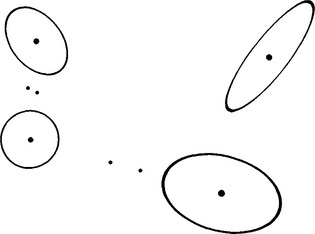
Figure 12.2 Result of using the basic diameter bisection method. The large dots show true ellipse centers found by the method, while the smaller dots show positions at which false alarms commonly occur. Such false alarms are eliminated by applying the test described in the text.
To proceed, the set of edge points that contribute to a given peak in parameter space is used to construct a histogram of R values (the latter being obtained from equation (12.1)). If a significant peak is found in this histogram, then we have clear evidence of an ellipse at the specified location in the image. If two or more such peaks are found, then we have evidence of a corresponding number of concentric ellipses in the image. If, however, no such peaks are found, then a rectangle, oval, or other symmetrical shape may be present, and each of these would need its own identifying test.
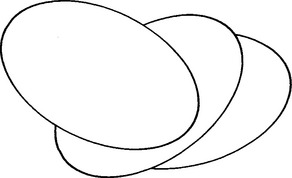
Clearly, then, the method relies on the existence of an appreciable number of pairs of edge points on an ellipse lying at opposite ends of diameters. Hence, strict limits are imposed on the amount of the boundary that must be visible (Fig. 12.3). Finally, it should not go unnoticed that the method wastes the signal available from unmatched edge points. These considerations have led to a search for further methods of ellipse detection.
12.3 The Chord-Tangent Method
The chord-tangent method was devised by Yuen et al. (1988) and makes use of another simple geometric property of the ellipse. Again, pairs of edge points are taken in turn, and for each point of the pair, tangents to the ellipse are constructed and found to cross at T; the midpoint of the connecting line is found at M; then the equation of the line TM is found and all points that lie on the portion MK of this line are accumulated in parameter space (Fig. 12.4). (Clearly, T and the center of the ellipse lie on the opposite sides of M.) Finally, peak location proceeds as before.
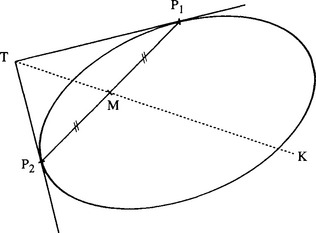
Figure 12.4 Principle of the chord-tangent method. The tangents at P1 and P2 meet at T and the midpoint of P1P2 is M. The center C of the ellipse lies on the line TM produced. Notice that M lies between C and T. Hence, the transform for points P1 and P2 need only include the portion MK of this line.
The proof that this method is correct is trivial. Symmetry ensures that the method works for circles, and projective properties then ensure that it also works for ellipses. Under projection, straight lines project into straight lines, midpoints into midpoints, tangents into tangents, and circles into ellipses; in addition, it is always possible to find a viewpoint such that a circle can be projected into a given ellipse.
Unfortunately, this method suffers from significantly increased computation, since so many points have to be accumulated in parameter space. This is obviously the price to be paid for greater applicability. However, computation can be minimized in at least three ways: (1) cutting down the lengths of the lines of votes accumulated in parameter space by taking account of the expected sizes and spacings of ellipses; (2) not pairing edge points initially if they are too close together or too far apart; and (3) eliminating edge points once they have been identified as belonging to a particular ellipse. (The last two techniques are also applicable to the diameter bisection method.)
Section 12.5 explores in more detail whether computation can be saved by reverting to the GHT approach. Meanwhile, it is necessary to consider how ellipse detection can be augmented by suitable procedures for finding ellipse orientation, size, and shape.
12.4 Finding the Remaining Ellipse Parameters
Although it has proved possible to locate ellipses in digital images by simple geometric constructions based on well-known properties of the ellipse, a more formal approach is required to determine other ellipse parameters. Accordingly, we write the equation of an ellipse in the form:
an ellipse being distinguished from a hyperbola by the additional condition:
This condition guarantees that A can never be zero and that the ellipse equation may, without loss of generality, be rewritten with A = 1. In any case, only ratios between the parameters have physical significance. This leaves five parameters, which can be related to the position of the ellipse, its orientation, and its size and shape (or eccentricity).
Having located the center of the ellipse, we may select a new origin of coordinates at its center (xc, yc). The equation then takes the form:
It now remains to fit to equation (12.4) the edge points that gave evidence for the ellipse center under consideration. The problem will in general be vastly overdetermined. Hence, an obvious approach is the method of least squares. Unfortunately, this technique tends to be very sensitive to outlier points and is therefore liable to be inaccurate. An alternative is to employ some form of Hough transformation. Since Hough parameter spaces require storage that increases exponentially with the number of unknown parameters, it is tempting to try to separate the determination of some of the parameters from that of others. For example, we can follow Tsukune and Goto (1983) by differentiating equation (12.4):
Then dy’/dx’ can be determined from the local edge orientation at (x’,y’) and a set of points accumulated in the new (H, B) parameter space. When a peak is eventually located in (H, B) space, the relevant data (a subset of a subset of the original set of edge points) can again be used with equation (12.4) to obtain a histogram of C’ values, from which the final parameter for the ellipse can be obtained.
The following formulas must be used to determine the orientation and semiaxes values of an ellipse in terms of H, B, and C :
Mathematically, 6 is the angle of rotation that diagonalizes the second-order terms in equation (12.4). Having performed this diagonalization, we find that the ellipse is essentially in the standard form ![]() , so a and b are determined.
, so a and b are determined.
This method finds the five ellipse parameters in three stages: first the positional coordinates are obtained, then the orientation, and finally the size and eccentricity.1This three-stage calculation involves less computation but compounds any errors–in addition, edge orientation errors, though low, become a limiting factor. For this reason, Yuen et al. (1988) tackled the problem by speeding up the HT procedure itself rather than by avoiding a direct assault on equation (12.4). That is, they aimed at a fast implementation of a thoroughgoing second stage, which finds all the parameters of equation (12.4) in one 3-D parameter space. Their fast adaptive HT procedure has already been described in Chapter 11 and is not covered again here.
At this stage it is clear that reasonably optimal means are available for finding the orientation and semiaxes of an ellipse once its position is known. The weak point in the process appears to be that of finding the ellipse initially. Indeed, the two approaches for achieving this that have been described above are particularly computationally intensive, mainly because they examine all pairs of edge points. Hence, we should again consider the GHT approach, which locates objects by taking edge points singly, to see whether any gains can be achieved by this means.
12.5 Reducing Computational Load for the Generalized Hough Transform Method
The complications described in Chapter 11 when the GHT is used to detect anisotropic objects clearly apply to ellipse detection. The various possible orientations of the object lead to the need to employ a large number of planes in parameter space. So far this chapter has avoided considering the GHT for these reasons. However, it will be seen that by accumulating the votes for all possible orientations in a single plane in parameter space, significant savings in computation can frequently be made. Basically, the idea is largely to eliminate the enormous storage requirements of the GHT by using only one instead of 360 planes in parameter space, while at the same time reducing by a large factor the computation involved in the final search for peaks. Such a scheme may have concomitant disadvantages such as the production of spurious peaks, and this aspect will have to be examined carefully.
To achieve these aims, it is necessary to analyze the shape of the point spread function (PSF) to be accumulated for each edge pixel, in the case of an ellipse of unknown orientation. We start by taking a general edge fragment at a position defined by ellipse parameter and deducing the bearing of the center of the ellipse relative to the local edge normal (Fig. 12.5). Working first in an ellipse-based axes system, for an ellipse with semimajor and semiminor axes a and b, respectively, it is clear that:
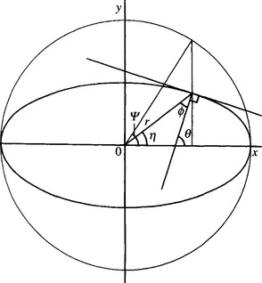
Hence, the orientation of the edge normal is given by:
At this point we wish to deduce the bearing φ of the center of the ellipse relative to the local edge normal. From Fig. 12.5:
 (12.18)
Substituting for tan 6 and tan η, and then rearranging, gives:
To obtain the PSF for an ellipse of unknown orientation, we now simplify matters by taking the current edge fragment to be at the origin and oriented with its normal along the u-axis (Fig. 12.6). The PSF is then the locus of all possible positions of the center of the ellipse. To find its form, it is necessary merely to eliminate ψ between equations (12.19) and (12.20). This is facilitated by reexpressing r2 in double angles (the significance of double angles lies in the 180° rotation symmetry of an ellipse):
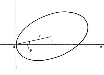
Figure 12.6 Geometry for finding the PSF for ellipse detection by forming the locus of the centers of ellipses touching a given edge fragment.
After some manipulation the locus is obtained as:
which can, in the edge-based coordinate system, also be expressed in the form:
Unfortunately, this is not a circle and is not even symmetrical about axes through its center. The shape of the PSF for various values of a and b is shown in Fig. 12.7. For very highly eccentric ellipses, the PSF is approximated by the arcs of two circles, one of radius a and the other of radius a2/b. It will be seen that in the other extreme, ellipses of low eccentricity, the PSF is approximated by an ellipse. In general, however, it is easy to see that, since the original ellipse possesses regions along the principal axes where the radii of curvature are approximately constant with values a2/b and b2/a, the PSF also possesses regions at either end of one diameter where the radii of curvature are (a2/b) –b and a– (b2/a). This makes it clear that the shape is not symmetrical and that it should become approximately symmetrical when a ![]() b.
b.
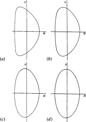
Figure 12.7 Typical PSF shapes for detection of ellipses with various eccentricities: (a) ellipse with a/b = 21.0, c/d = 1.1; (b) ellipse with a/b = 5.0, c/d = 1.5; (c) ellipse with a/b = 2.0, c/d = 3.0; (d) ellipse with a/b = 1.4, c/d = 6.0. Notice how the PSF shape approaches a small ellipse of aspect ratio 2.00 as eccentricity tends to zero. The semimajor and semiminor axes of the PSF are 2d and d, respectively.
and then taking an approximation of small d, the locus is obtained in the form:
Neglecting the term d 2/2c which provides a small correction to u, the PSF is itself approximately an ellipse of semimajor axis 2d and semiminor axis d. Making use of this fact simplifies implementation, but it is practicable only for low-eccentricity ellipses where d ![]() 0.1c, so that a
0.1c, so that a ![]() 1.2b. In practice, however, where ellipses are small and the PSF is only a few pixels across, it is a reasonable approximation to insist only that a< 2b.
1.2b. In practice, however, where ellipses are small and the PSF is only a few pixels across, it is a reasonable approximation to insist only that a< 2b.
Implementation is simplified since a universal lookup table (ULUT) for ellipse detection can be compiled, which is independent of the size and eccentricity of the ellipse to be detected as long as the eccentricity is not excessive. Since ellipses are common features in industrial and other applications–arising both from elliptical objects and from oblique views of circles–this factor should be an important consideration in many applications. Thus, a single ULUT is compiled and stored, and it then needs only to be scaled and positioned to produce the PSF in a given instance of ellipse detection.
12.5.1 Practical Details
Having constructed a ULUT for ellipse detection, we find that the detection algorithm has to scale it, position it and rotate it so that points can be accumulated in parameter space. A priori, it would be imagined that a considerable amount of trigonometric computation is involved in this process. However, it is possible to avoid calculating angles directly (e.g., using the arctan function) by always working with sines and cosines. This is rendered possible partly because such edge orientation operators as the Sobel give two components (gx, gy) for the intensity gradient vector. (This has now been seen to happen in several line and circle detection schemes–see Chapters 9 and 10.) Hence, a considerable amount of computation can be saved, as is demonstrated by the simplicity of the final code for computing a given contribution to the PSF (Fig. 12.8).
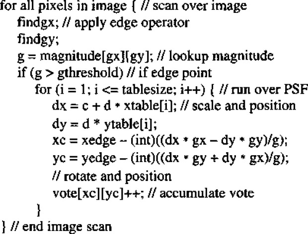
Figure 12.8 Algorithm for ellipse detection. In this section of code, it is arbitrarily (i) that the magnitude of the vector (gx, gy) is available from a lookup table, and (ii) that all calculations are carried out in floating-point form until the final “rounding” stage where voting positions are being estimated to the nearest pixel.
Figure 12.9 shows the result of testing the above scheme on an image of some O-rings lying on a slope of arbitrary direction. The O-rings are found accurately and with a fair degree of robustness–that is, despite overlapping and partial occlusion (up to 40% in one case). In several cases, incidental transforms from points on the inner edges of the O-rings overlap other transforms from points on the outer edges, although only the latter are actually employed usefully here for peak finding. Hence, the scheme is able to overcome problems resulting from additional clutter in parameter space.
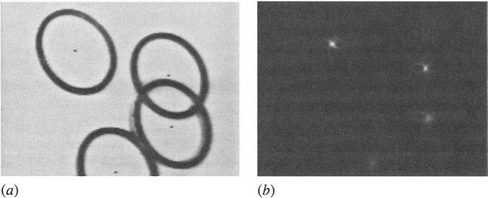
Figure 12.9 Applying the PSF to detection of tilted circles: (a) off-camera 128 × 128 image of a set of circular O-rings on a 45° slope of arbitrary direction; (b) transform in parameter space. Notice the peculiar shape of the ellipse transform, which is close to a “four-leaf clover” pattern. (a) also indicates the positions of the centers of the O-rings as located from (b): accuracy is limited by the presence of noise, shadows, clutter, and available resolution, to an overall standard deviation of about 0.6 pixel.
Figure 12.9 also shows the arrangement of points in parameter space that results from applying the PSF to every edge point on the boundary of an ellipse. The pattern is somewhat clearer in Fig. 12.10. In either case it is seen to contain a high degree of structure. For an ideal transform, there would be no structure apart from the main peak. Looking at the situation in another way, in deducing the locus of points forming the PSF we found all points that could possibly be at the center of an ellipse when we had no knowledge about its orientation. All points on the PSF not falling on the peak at the center of the ellipse would hopefully be randomly (and fairly uniformly) distributed nearby. However, for a shape such as an ellipse–which has a particular structure and symmetry of its own–this is not the situation. A full computation of the positions of votes in parameter space yields many candidate positions, and to find strong structure in the transform it is necessary to look for envelopes to the system of PSFs.
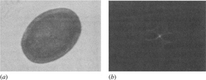
Figure 12.10 Applying the PSF to detection of elliptical objects: (a) off-camera 128 × 128 image of an elliptical bar of soap of arbitrary orientation; (b) transform in parameter space. In this case, the clover-leaf pattern is better resolved. Accuracy of location is limited partly by distortions in the shape of the object, but the peak location procedure results in an overall standard deviation of the order of 0.5 pixel.
This is a sufficiently complex task to be left to experiment, but one or two observations on the results are useful and relevant. First, where there is a lot of local symmetry in the starting shape (the ellipse)–and specifically where the curvature on the boundary is approximately constant–this leads automatically to strong envelope lines in the transform, as indicated in Fig. 12.11, where the onaxes regions of the original ellipse have essentially been moved radially (and are hence also compressed laterally) until they pass through its center. These lines seem practically to form a “four-leaf clover” pattern, although the loops become more diffuse on moving away from the center, in accordance with the envelope idea expressed above.
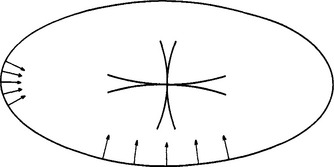
Figure 12.11 Formation of the ellipse transform by moving the regions of the ellipse boundary lying roughly along the principal axes radially inward until they pass through the center of the ellipse. The reason for this peculiar construction lies in the fact that the prominent lines in the transform are the envelopes of all possible PSFs. The necessary coherence is provided by the nearly constant radii of curvature roughly along the directions of the principal axes.
The important problem here is whether the structure in the transform is misleading–that is, whether it gives rise to sharply focused peaks at other positions than the main peak. This does not appear to happen, the main and most intense structure being the cross pattern at the center. This pattern is clearly strongest and most focused (both practically and theoretically) near the center, while, in addition, it goes up to double the height quite sharply as the two branches cross at the very center. The overall conclusion is that the additional structure does no particular harm, although it gives rise to interesting complications iftwo ellipses overlap so that their centers are quite close. Hence, it is more difficult to use the method described here to disentangle two such ellipses than it would be to disentangle two circular objects with a similar degree of overlap. The way around this problem is to check individual high points in the transform by interrogating the original image. See, for example, Bolles and Cain (1982), Davies (1987g), and Chapters 13 and 15.
More help would be obtained in interpreting the transform in such cases if the PSFs were regarded not as mere loci of the centers of ellipses of different orientations touching a given edge fragment, but as loci with proper weights, unit weight corresponding to unit boundary distance on the original ellipse. This is too complex a problem to be pursued here, but it may be noted that curvature information immediately leads to the prediction of larger weights for the part of the PSF corresponding to the two regions of the ellipse along the minor axes.
Finally, note that accuracy will be lost if the PSF is not guaranteed to place a vote at the center of the ellipse for every edge pixel. This means that the PSF should be a connected chain of pixels. Hence, the size of the lookup table (LUT) must vary with the size of the PSF. Or, if a large ULUT is used, a small PSF should be able to skip over a proportion of the entries. In the examples of Figs. 12.9 and 12.10, the PSF contained 50 and 100 votes, respectively.
12.6 Comparing the Various Methods
To compare the computational loads for the methods of ellipse detection discussed above, we concentrate on ellipse location per se and ignore any additional procedures concerned with (1) finding other ellipse parameters, (2) distinguishing ellipses from other shapes, or (3) separating concentric ellipses. We start by examining the GHT method and the diameter bisection method.
First, suppose that an N × N pixel image contains p ellipses of identical size given by the parameters a, b, c, d as defined in Section 12.3. By ignoring noise and general background clutter, we shall be favoring the diameter bisection method, as will be seen below. Next, the discussion is simplified by supposing that the computational load resides mainly in calculating the positions at which votes should be accumulated in parameter space–the effort involved in locating edge pixels and in locating peaks in parameter space is much smaller.
Under these circumstances, the load for the GHT method may be approximated by the product of the number of edge pixels and the number of points per edge pixel that have to be accumulated in parameter space, the latter being equal to the number of points on the PSF. Hence, the load is proportional to:
 (12.27)
where the ellipse has been taken to have relatively low eccentricity so that the PSF itself approximates to an ellipse of semiaxes 2d and d.
For the diameter bisection method, the actual voting is a minor part of the algorithm–as indeed it is in the GHT method (see the snippet of code listed in Fig 12.8). In either case, most of the computational load concerns edge orientation calculations or comparisons. Assuming that these calculations and comparisons involve similar inherent effort, we may fairly assess the load for the diameter bisection method as:
 (12.28)
When a is close to b, as for a circle, LA → 0, and then the diameter bisection method becomes a very poor option. In many cases, however, a is close to 2b,so that c is close to 3d. The ratio of the loads then becomes:
It is possible that p will be as low as 1 in some cases. Such cases are likely to be rare, however, and are offset by applications where there is significant background image clutter and noise, or where all p ellipses have other edge detail giving irrelevant signals that can be considered as a type of self-induced clutter (see the O-ring example of Fig. 12.9). The overall image “clutter factor” would normally be expected to be at least two.
It is also possible that some of the pairs of edge points in the diameter bisection method can be excluded before they are considered, for example, by giving every edge point a range of interaction related to the size of the ellipses. This would tend to reduce the computational load by a factor of the order of (but not as small as) p. However, the computational overhead required for this would not be negligible.
Overall, the GHT method will no doubt be significantly faster than the diameter bisection method in most real applications, the diameter bisection method being at a definite disadvantage when image clutter and noise is strong. The only situation where the diameter bisection method might win appears to be when an image contains a minimal number of highly eccentric ellipses. By comparison, the chord-tangent method always requires more computation than the diameter bisection method, since not only does it examine every pair of edge points but also it generates a line of votes in parameter space for each pair.
Against these computational limitations must be noted the different characteristics of the methods. First, the diameter bisection method is not particularly discriminating in that it locates many symmetrical shapes, as remarked earlier. The chord-tangent method is selective for ellipses but is not selective about their size or eccentricity. The GHT method is selective about all of these factors. These types of discriminability, or lack of it, can turn out to be advantageous or disadvantageous, depending on the application. Hence, we do no more here than draw attention to these different properties. It is also relevant that the diameter bisection method is rather less robust than the other methods. This is so because if one edge point of an antiparallel pair is not detected, then the other point of the pair cannot contribute to detection of the ellipse–a factor that does not apply for the other two methods since they take all edge information into account.
12.7 Concluding Remarks
The simplest scheme for ellipse detection in digital images is the diameter bisection method, which, unfortunately, is not very robust because many pairs of diameter ends need to be visible before sufficient signal can be built up. One alternative is the chord-tangent method; this is highly robust, yet at the penalty of considerable additional computation. Another alternative is the GHT, but when applied to anisotropic shapes this method requires that one plane in parameter space be used for each discriminable orientation of the shape. However, if a single plane parameter space is used for this purpose, the GHT approach frequently requires less computational effort than the other two methods. This is because they are based on using pairs of edge points to deduce candidate ellipse centers, whereas the GHT takes edge points one at a time. However, the three methods differ markedly in their shape discriminability characteristics, as should be noted in real applications.
In particular, the diameter bisection method locates ellipses of all eccentricities, sizes, and orientations, and also other symmetrical shapes; the chord-tangent method locates ellipses of all eccentricities, sizes, and orientations but discriminates against other shapes; and the GHT locates ellipses of all orientations but discriminates against ellipses of the wrong eccentricity and size and against other shapes. However, the GHT can be adapted to detect many other shapes, whereas the diameter bisection method is limited and the chord-tangent method is specific to ellipses.
With the GHT, the avoidance of many planes in parameter space is one aspect of a more general problem. For example, we might need to use many planes in parameter space to allow for variation in object size. It is also possible that we might know the size and orientation of an ellipse but not its eccentricity, many planes being needed to cope with this situation. In Chapter 10 it was shown that circles of many sizes can be sought simultaneously in a single plane in parameter space, by a method related to that described here (viz., using a PSF consisting of a radial line in place of a single point). It is clear that this method will carry over to ellipses and other shapes (i.e., replace the R (θ) in the basic transform in turn by αR (θ), for all a in a given range, leaving φ(θ) unchanged). Similarly, it is evident from the derivation in Section 12.5 that the GHT approach carries over to other shapes when orientation is unknown.
Finally, a similar extension can be made when eccentricity is unknown but size and orientation are known. Thus, we hypothesize generally that parameter space can be compressed by one degree of freedom from the ideal in order to save computation. We also note that it is not possible to compress parameter space by more than one degree of freedom from the ideal. If we tried to do this, virtually any shape would be able to trigger the detector and there would be a great many false alarms. As an example, if we try to detect ellipses of unknown orientation and size in a single plane in parameter space, the PSF becomes an extended blob that is unable to discriminate between a great variety of shapes. (In general, the PSF becomes an area that is the result of convolving the two basic PSF curves in parameter space. Indeed, it is not possible to find two such curves that do not produce an area when convolved.) These observations appear both to extend and ultimately to limit the capabilities of the GHT approach for object location, and they are by no means limited to ellipse detection.
12.8 Bibliographical and Historical Notes
This chapter is based on relatively few papers: first, that of Tsuji and Matsumoto (1978), whose insight led to a totally new ellipse detector; second, that of Tsukune and Goto (1983), which aimed at more accurate determination of ellipse parameters; third, that of Yuen et al. (1988), whose detector made good certain shortcomings of the previous two methods; and fourth, that of Davies (1989a), who developed the GHT idea of Ballard (1981) in order to save computation. The contrasts between these methods are many and intricate, as the chapter has shown. In particular, the idea of saving dimensionality in the implementation of the GHT appears also in a general circle detector (Davies, 1988b). At that point in time, the necessity for a multistage approach to determine ellipse parameters seemed proven, although somewhat surprisingly the optimum number of such stages was just two.
Later algorithms represented moves to greater degrees of robustness with real data by explicit inclusion of errors and error propagation (Ellis et al., 1992). Greater attention was subsequently given to the verification stage of the Hough approach (Ser and Siu, 1995). In addition, work was carried out on the detection of superellipses, which are shapes intermediate in shape between ellipses and rectangles, though the technique used (Rosin and West, 1995) was that of segmentation trees rather than Hough transforms. (Nonspecific detection of superellipses can, of course, be achieved by the diameter bisection method; see Section 12.2.). See also Rosin (2000).
Most recently, ultrafast algorithms were needed for cereal grain inspection–flow rates in excess of 300 grains per second being typical–and the resulting algorithms were limiting cases of chord-based versions of the Hough transform (Davies, 1999b,e). A related approach was adopted by Xie and Ji (2002) for their efficient ellipse detection method. Lei and Wong (1999) employed a method that was based on symmetry and was found to be able to detect parabolas and hyperbolas as well as ellipses.2
It was also reported as being more stable than other methods since it does not have to calculate tangents or curvatures; Sewisy and Leberl (2001) have also reported this advantage. Wang and Sung (2001) applied the Hough transform to eye gaze determination by location of irises. They found that the method had to be refined sufficiently to detect the irises as ellipses, not only because of iris orientation but also because the shape of the eye is far from spherical and the horizontal diameter is larger than the vertical diameter.
The fact that even in the 2000s, basic new ellipse detection schemes are being developed says something about the science of image analysis. Even today the toolbox of algorithms is incomplete, and the science of how to choose between items in the toolbox, or how, systematically, to develop new items for the toolbox, is immature. Furthermore, although all the parameters for specification of such a toolbox may be known, knowledge about the possible tradeoffs between them is still at an early stage.
12.9 Problems
1. Derive equations (12.7)-(12.9) by the method suggested in the text.
2. Determine which of the methods described in this chapter will detect (a) hyperbolas, (b) curves of the form Ax3 + By3 = 1, and (c) curves of the form Ax4 + Bx + Cy4 = 1.
3. Prove equation (12.1) for an ellipse. Hint: Write the coordinates of P and Q in suitable parametric forms, and then use the fact that OP ⊥ OQ to eliminate one of the parameters from the left-hand side of the equation.
4. Describe the diameter-bisection and chord-tangent methods for the location of ellipses in images, and compare their properties. Justify the use of the chord-tangent method by proving its validity for circle detection and then extending the proof to cover ellipse detection.
5. Round coins of a variety of sizes are to be located, identified, and sorted in a vending machine. Discuss whether the chord-tangent method should be used for this purpose instead of the usual form of Hough transform circle location scheme operating within a 3-D (x, y, r) parameter space.
6. Outline each of the following methods for locating ellipses using the Hough transform: (a) the diameter-bisection method; (b) the chord-tangent method. Explain the principles on which these methods rely. Determine which is the more robust and compare the amounts of computation each requires.
7. For the diameter-bisection method, searching through lists of edge points with the right orientations can take excessive computation. It is suggested that a two-stage approach might speed up the process: (a) load the edge points into a table that may be addressed by orientation; (b) look up the right edge points by feeding appropriate orientations into the table. Estimate how much this would be likely to speed up the diameter-bisection method.
8. It is found that the diameter-bisection method sometimes becomes confused when several ellipses appear in the same image and generate false “centers” that are not situated at the centers of any ellipses. It is also found that certain other shapes are detected by the diameter-bisection method. Ascertain in each case what the method is sensitive to and consider ways in which these problems might be overcome.