7.2. Quotient Space Approximation and Second-Generation Wavelets
Since the quotient space approximation is a multi-resolution analysis method, it is closely related to wavelets analysis. Now, we discuss their connection.
7.2.1. Second-Generation Wavelets Analysis
We can see the wavelet transform (WT) as a decomposition of a signal f(x) onto a set of basis functions called wavelets to obtain a series expansion of the signal. So far there are two kinds of WT, the first-generation wavelets (Mallat, 1989; Rioul and Vetterli, 1991; Unser and Blu, 2003) and the second-generation wavelets (Sweldens, 1998). In the first-generation wavelets, the basis functions are obtained from a single mother wavelet by dilations and translations. Then, the signal f(x) is directly projected onto the basis functions by taking the inner product between f(x) and the functions. If a set of basis functions is obtained from dilating and translating the mother wavelet, the function becomes spread out in time, then the corresponding projection onto the set of basis functions takes only the coarse resolution structure of f(x) into account. This implies that this set of basis functions composes a coarse space. Conversely, if a set of basis functions is obtained from contracting and translating the mother wavelet, the fine structure of f(x) will be taken. It means that this set of basis functions composes a fine space.
Now, we introduce Haar wavelet as follows, where X is a measurable subset in an n-dimensional European space.
Definition 7.11
General Haar Wavelet
Definition 7.12
Definition 7.13
Define a subspace  .
.
Definition 7.14
Assume that Wj is the orthogonal complement of Vj on Vj+1.  is an orthogonal base on Wj, is called a general Haar wavelet.
7.2.2. Quotient Space Approximation
1. Introduction
Since equivalence relation and spatial partition are mutually equivalent, a set of hierarchical quotient spaces, a set of hierarchical equivalence relations and a set of hierarchical partitions are equivalent. Namely, a series of finite hierarchical partitions in the second-generation wavelet is equivalent to the above as well.
We will show below that the quotient space approximation of signal f(x) corresponds to some sort of wavelet approximation.
2. Quotient Space Approximation
Recently, there are two forms for approximating (or decomposing) a signal f(x), the limit form  , and the series expansion
  . These two forms are equivalent. In wavelet transform, the signal is expanded into a series form. In the series expansion, only the increment of the signal values is represented at the high-resolution levels. The quotient space approximation of a given signal is based on the limit form. If transforming the limit form of quotient space approximation into the series expansion, we will have some sort of wavelet transforms.
Assume that f is an attribute function on X.  is a set of hierarchical quotient spaces on X. Define a quotient function
  , where
  denotes the mean of x. And we call the quotient function as a quotient function defined by the mean principle. Assume that
  is the (dyadic) quotient space of
  .
.
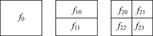
As shown in Fig. 7.1,  is the mean of
  on
on  .
.  and
and  are the means of at elements
  and
and  of
of  , respectively. For simplicity, assume that the measure of each equivalence class is the same, i.e.,
  . We may use
  to describe
  , or use the increment between () and to describe , for example, if
  , then
  and
and  . We may use
  to describe as well.
Assume that  . For , let
  . For , let
  . We have
  .
.
Generally, there are  equivalence classes in the i-th level and its corresponding mean is
  . Let
. Let
![]() (7.7)
(7.7)
We have
![]() (7.8)
(7.8)
Definition 7.15
The quotient space approximation process can also be described by the quotient incremental function.
3. The Relation between Two Quotient Space Approximation Forms
From Formula (7.7), we know that  can be computed from a known
  . We will show below that can be computed from the known and .
Definition 7.16
Assume that integer a is a binary number with n bits.  is the first j bits of a.
Example 7.3
Assume that  . Then,
  ,
,  ,
,  ,
,  , and
, and  . Therefore, an element of quotient space
  can be represented by a j-dimensional vector . Replacing each component with 0 value of by value –1, we have a new vector
  .
.
Definition 7.17
Example 7.4
![]()
![]()
![]()
Theorem 7.1
A function f on  and a set
  of hierarchical (dyadic) partitions are given.
  is a quotient function defined by the mean principle.
  is a quotient incremental function defined by Formula (7.7).
  is an
is an  -dimensional binary vector. Then
![]() (7.9)
(7.9)
Proof
By induction, when  , from the definition of
  , we have that Formula (7.9) holds. Assume that Formula (7.9) holds for
  , i.e.,
![]()
![]() (7.10)
(7.10)
Since
![]() (7.11)
(7.11)
Example 7.5
Find the f value of the 21st element at the 5th quotient space. Let a=(1,-1,1,-1,1)=21. And find the f value of the equivalence class that a belongs to at the 4th level.
Theorem 7.2
Assume that converges to X with respect to its grain-size, and quotient function  is constructed by the mean principle. If f is uniformly continuous on X, then converges to f with respect to the grain-size.
The theorem can be obtained from Proposition 7.1 directly.
Proposition 7.4
Proof
The coefficient of with respect to  is
is
The coefficient of with respect to  is
is
Theorem 7.3
If  is a series of quotient functions approximating to on
  , then
(1) The quotient function  at the
  -th level is the coefficient of the expansion of
  on scaling function base
  of the general Haar wavelet at the -th level (multi-resolution).
(2) The quotient incremental function  at the -th level is the coefficient of the expansion of on the general Haar wavelet base
  .
.
(3) Formula (7.9) is the transformation relation between quotient functions [f] and quotient incremental functions in the quotient space approximation.
It’s noted that although Formula (7.9) is obtained under the dyadic assumption, the similar but more complex result can be got in general cases. In multi-resolution analysis, the dyadic wavelet with n levels has  basis functions (wavelets), so the number of coefficients in the wavelet expansion of is . But in Formula (7.9), the number of coefficients is only n simply. Of course, the total number of values in is
  .
.
7.2.3. The Relation between Quotient Space Approximation and Wavelet Analysis
7.2.3.1. The Meaning of Wavelet Analysis
We will explain the physical significance of wavelet analysis from the quotient space approximation point of view. From Section 7.3,  is a quotient function obtained from refining space , or from adjusting function . It can also be represented by the quotient function on
  directly. If adding a quotient incremental function
  , then we have
  . By recursion, we have a series form
![]()
Generally,  .
.
From the multi-granular computing point of view, term  represents the variation of f, when the grain-size changing from the n-1-th level to the n-th level, i.e., the rate of change (frequency) at each grain-size. The finer the grain-size, or the bigger the n, the higher the changing frequency of
  . So is just the so-called ‘wavelet’. From a mathematical view point, when replacing the sequential convergence-based quotient space approximation by the series convergence-based one, ‘wavelet’ is an inevitable product. ‘Wavelet’ is the description of the difference between two adjacent quotient space approximations.
7.2.3.2. The Comparison between Wavelet and Quotient Space Approximation
In wavelet analysis, it’s needed to choose a set of complete, orthonormal basis functions in a functional space, and then a square-integrable function is represented by a wavelet series with respect to the base. The method allows the commonality across different applications. In quotient space approximation, for a given function, it’s needed to choose a specific domain partition method, and then to approximate the quotient functions (or quotient incremental functions). In the domain partition process, when the incremental value  of quotient functions in some equivalence class is rather large, the class is refined. When the value in some equivalence class is small enough, the partition stops. The partition can be adjusted dynamically. This ‘customized’ method is flexible and personalized. Therefore, in wavelet analysis, for a kind of functions, we need to choose a proper wavelet base that is difficult generally. In quotient space approximation, it’s only needed to construct a proper quotient function for a specific function that is an easier task.
7.2.3.3. Different Forms of Quotient Functions
In the above discussion, the quotient functions are defined by the mean of values of the given original function. The quotient functions can also be defined by the sum of values of the given original function.
Assume that f is a performance function on X. is a set of hierarchical quotient spaces. The sequence of quotient spaces is required to be dimidiate, not necessarily halved. Let quotient functions be
![]()
![]()
The corresponding quotient incremental functions  are defined as
![]() (7.12)
(7.12)
We have
![]()
![]() (7.13)
(7.13)
Definition 7.19
Define an i-dimensional vector as
![]()
Definition 7.20
Define an i-dimensional vector as
![]()
Proposition 7.5
Proof
Similar to the proof in Theorem 7.3, by recursion, the results can be obtained directly.
It’s noted that when the partition is not halved,  may be obtained by Formulas (7.12)–(7.14), and again
  and
and  may be obtained from Formula (7.15).
We show that the series form of quotient space approximation is equivalent to the second-generation wavelets. This means that many mature tools in wavelet analysis can be transformed to quotient space-based granular computing, for example, lifting scheme, fast lifting wavelet transform, etc.
Further, other methods in the second-generation wavelets can also be applied to performance, stability, robustness, and convergence analysis of systems besides the attribute functions that we have discussed.
..................Content has been hidden....................
You can't read the all page of ebook, please click here login for view all page.