
11.4.2 Adiabatic Tubular Reactor
We can rearrange Equation (11-29) to solve for temperature as a function of conversion; that is

This equation will be coupled with the differential mole balance
![]()
to obtain the temperature, conversion, and concentration profiles along the length of the reactor. The algorithm for solving PBRs and PFRs operated adiabatically using a first-order reversible reaction ![]() as an example is shown in Table 11-2.
as an example is shown in Table 11-2.
Table 11-3 gives two different methods for solving the equations in Table 11-2 in order to find the conversion, X, and temperature, T, profiles down the reactor. The numerical technique (e.g., hand calculation) is presented primarily to give insight and understanding to the solution procedure and this understanding is important. With this procedure one could either construct a Levenspiel plot or use a quadrature formula to find the reactor volume. It is doubtful that anyone would actually use either of these methods unless they had absolutely no access to a computer and they would never get access (e.g., stranded on a desert island with a dead laptop satellite connection). The solution to reaction engineering problems today is to use software packages with ordinary differential equation (ODE) solvers, such as Polymath, MATLAB, or Excel, to solve the coupled mole balance and energy balance differential equations.
Table 11-2. Adiabatic PFR/PBR Algorithm
The elementary reversible gas-phase reaction
![]()
is carried out in a PFR in which pressure drop is neglected and pure A enters the reactor.
Mole Balance:
![]()
Rate Law:
![]()
with
![]()
and for ΔCP = 0
![]()
Stoichiometry: Gas, ε = 0, P = P0
![]()
![]()
Combine:
![]()
Energy Balance:
To relate temperature and conversion, we apply the energy balance to an adiabatic PFR. If all species enter at the same temperature, Ti0 = T0.
Solving Equation (11-29), with ![]() ,
, ![]() , to obtain T as a function of conversion yields
, to obtain T as a function of conversion yields
![]()
If pure A enters and iff ΔCP = 0, then
![]()
Equations (T11-2.1) through (T11-2.9) can easily be solved using either Simpson’s rule or an ODE solver.
Table 11-3. Solution Procedures for Adiabatic PFR/PBR Reactor
A. Numerical Technique
Integrating the PFR mole balance,
Choose X → Calculate T → Calculate k → Calculate –rA → Calculate ![]()
T11-3.1
![]()
The numerical technique is presented to provide insight to how the variables (k, Kc, etc.) change as we move down the reactor from V = 0 and X = 0 to Vf and Xf.
- Set X = 0.
- Calculate T using Equation (T11-2.9).
- Calculate k using Equation (T11-2.3).
- Calculate kC using Equation (T11-2.4).
- Calculate T0/T (gas phase).
- Calculate –rA using Equation (T11-2.7).
- Calculate (FA0/ – rA).
- If X is less than the exit conversion X3 specified, increment X (i.e., Xi + I = Xi + ΔX) and go to Step 2.
- Prepare table of X vs. (FA0/–rA).
- Use numerical integration formulas given in Appendix A, for example,
T11-3.2

with

Use evaluation techniques discussed in Chapter 2.
B. Ordinary Differential Equation (ODE) Solver
We will now apply the algorithm in Table 11-2 and solution procedure B in Table 11-3 to a real reaction.
Example 11-3. Adiabatic Liquid-Phase Isomerization of Normal Butane
Normal butane, C4H10, is to be isomerized to isobutane in a plug-flow reactor. Isobutane is a valuable product that is used in the manufacture of gasoline additives. For example, isobutane can be further reacted to form iso-octane. The 2010 selling price of n-butane was $0.44/kg, while the trading price of isobutane was $0.68/kg.

This elementary reversible reaction is to be carried out adiabatically in the liquid phase under high pressure using essentially trace amounts of a liquid catalyst which gives a specific reaction rate of 31.1 h–1 at 360 K. The feed enters at 330 K.
a. Calculate the PFR volume necessary to process 100,000 gal/day (163 kmol/h) at 70% conversion of a mixture 90 mol % n-butane and 10 mol % i-pentane, which is considered an inert.
b. Plot and analyze X, Xe, T, and –rA down the length of the reactor.
c. Calculate the CSTR volume for 40% conversion.
Additional information:
![]() = –6900 J/mol n-butane, Activation energy = 65.7 kJ/mol KC = 3.03 at 60°C, CA0 = 9.3 mol/dm3 = 9.3 kmol/m3
= –6900 J/mol n-butane, Activation energy = 65.7 kJ/mol KC = 3.03 at 60°C, CA0 = 9.3 mol/dm3 = 9.3 kmol/m3

![]()
a. PFR algorithm
- Mole Balance:
E11-3.1

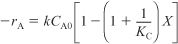
- Rate Law:
E11-3.2

with
E11-3.3

E11-3.4

- Stoichiometry (liquid phase, υ = υ0):
E11-3.5

E11-3.6


- Combine:
E11-3.7

- Energy Balance: Recalling Equation (11-27), we have
11-27

From the problem statement

Applying the preceding conditions to Equation (11-27) and rearranging gives
E11-3.8

- Parameter Evaluation:
E11-3.9

where T is in degrees Kelvin.
Substituting for the activation energy, T1, and k1 in Equation (E11-3.3), we obtain
E11-3.10

Substituting for
 , T2, and KC(T2) in Equation (E11-3.4) yields
E11-3.11

Recalling the rate law gives us
E11-3.7
- Equilibrium Conversion:
At equilibrium
–rA ≡ 0
and therefore we can solve Equation (E11-3.7) for the equilibrium conversion
E11-3.12

Because we know KC(T), we can find Xe as a function of temperature.

PFR Solution
a. Find the PFR volume necessary to achieve 70% conversion. This problem statement is risky. Why? Because the adiabatic equilibrium conversion may be less than 70%! Fortunately, it’s not for the conditions here 0.7 < Xe. In general, we should ask for the reactor volume to obtain 95% of the equilibrium conversion, Xf = 0.95 Xe.
b. Plot and analyze X, Xe, –rA, and T down the length (volume) of the reactor.
We will solve the preceding set of equations to find the PFR reactor volume using both hand calculations and an ODE computer solution. We carry out the hand calculation to help give an intuitive understanding of how the parameters Xe and –rA vary with conversion and temperature. The computer solution allows us to readily plot the reaction variables along the length of the reactor and also to study the reaction and reactor by varying the system parameters such as CA0 and T0.
Part (a) [Solution by Hand Calculation to perhaps give greater insight and to build on techniques in Chapter 2.]
We will now integrate Equation (E11-3.8) using Simpson’s rule after forming a table (E11-3.1) to calculate (FA0/–rA) as a function of X. This procedure is similar to that described in Chapter 2. We now carry out a sample calculation to show how Table E11-3.1 was constructed.
For example, at X = 0.2.
a. T = 330 + 43.4(0.2) = 338.6 K
b. ![]()
c. ![]()
d. ![]()
e. ![]()
Sample calculation for Table E11-3.1
f. ![]()
Table E11-3.1. Hand Calculation

Continuing in this manner for other conversions, we can complete Table E11-3.1.
Use the data in Table E11-3.1 to make a Levenspiel plot, as in Chapter 2.
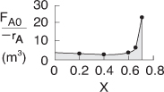
The reactor volume for 70% conversion will be evaluated using the quadrature formulas. Because (FA0/–rA) increases rapidly as we approach the adiabatic equilibrium conversion, 0.71, we will break the integral into two parts.
E11-3.13
![]()
Using Equations (A-24) and (A-22) in Appendix A, we obtain

Why are we doing this hand calculation? If it isn’t helpful, send me an email and you won’t see this again.
You probably will never ever carry out a hand calculation similar to the one shown above. So why did we do it? Hopefully, we have given the reader a more intuitive feel of the magnitude of each of the terms and how they change as one moves down the reactor (i.e., what the computer solution is doing), as well as to show how the Levenspiel Plots of (FA0/–rA) vs. X in Chapter 2 were constructed. At the exit, V = 2.6 m3, X = 0.7, Xe = 0.715, and T = 360 K.
Part (b) PFR computer solution and variable profiles
We could have also solved this problem using Polymath or some other ODE solver. The Polymath program using Equations (E11-3.1), (E11-3.7), (E11-3.9), (E11-3.10), (E11-3.11), and (E11-3.12) is shown in Table E11-3.2.
Table E11-3.2. Polymath Program Adiabatic Isomerization

Analysis: The graphical output is shown in Figure E11-3.1. We see from Figure E11-3.1(c) that 1.15 m3 is required for 40% conversion. The temperature and reaction rate profiles are also shown. Notice anything strange? One observes that the rate of reaction

Figure E11-3.1. Adiabadic PFR temperature, reaction rate, and conversion profiles.
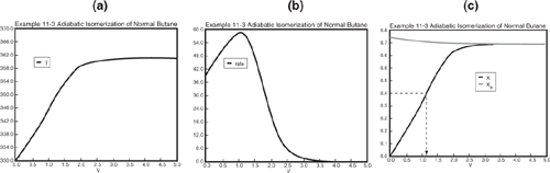
Look at the shape of the curves in Figure E11-3.1. Why do they look the way they do?
goes through a maximum. Near the entrance to the reactor, T increases as does k, causing term A to increase more rapidly than term B decreases, and thus the rate increases. Near the end of the reactor, term B is decreasing more rapidly than term A is increasing. Consequently, because of these two competing effects, we have a maximum in the rate of reaction.
AspenTech: Example 11-3 has also been formulated in AspenTech and can be loaded on your computer directly from the DVD-ROM.

Let’s now calculate the adiabatic CSTR volume necessary to achieve 40% conversion. Do you think the CSTR will be larger or smaller than the PFR? The mole balance is
![]()
Using Equation (E11-3.7) in the mole balance, we obtain

From the energy balance, we have Equation (E11-3.10):
For 40% conversion
T = 330 + 43.4X
T = 330 + 43.4(0.4) = 347.3K
Using Equations (E11-3.11) and (E11-3.12) or from Table E11-3.1,
k = 14.02 h–1
KC = 2.73
Then

We see that the CSTR volume (1 m3) to achieve 40% conversion in this adiabatic reaction is less than the PFR volume (1.15 m3).
One can readily see why the reactor volume for 40% conversion is smaller for a CSTR than a PFR by recalling the Levenspiel plots from Chapter 2. Plotting (FA0/–rA) as a function of X from the data in Table E11-3.1 is shown here.

The PFR area (volume) is greater than the CSTR area (volume).
Analysis: In this example we applied the CRE algorithm to a reversible-first-order reaction carried out adiabatically in a PFR and in a CSTR. We note that at the CSTR volume necessary to achieve 40% conversion is smaller than that to achieve the same conversion in a PFR. In Figure E11-3.1(c) we also see that at a PFR volume of three m3, equilibrium is essentially reached about half way through the reactor, and no further changes in temperature, reaction rate, equilibrium conversion, or conversion take place further down the reactor.
11.5 Adiabatic Equilibrium Conversion and Reactor Staging
The highest conversion that can be achieved in reversible reactions is the equilibrium conversion. For endothermic reactions, the equilibrium conversion increases with increasing temperature up to a maximum of 1.0. For exothermic reactions, the equilibrium conversion decreases with increasing temperature.