
Chapter 18. Images and Signal Processing
18.1. Introduction
This chapter introduces the mathematics needed to understand what happens when we perform various operations on images like scaling, rotating, blurring, sharpening, etc., and how to avoid certain unpleasant artifacts when we do these operations. It’s a long chapter with lots of mathematics; we’ve done our best to keep it to a minimum without telling any lies. We begin with a very concise summary of the chapter, and gradually expand on the themes presented there.
The entire chapter can be regarded as an application of the Coordinate-System/Basis principle: Always use a basis that is well suited to your work. In this case, the objects we’re working with are not geometric shapes, as in Chapter 2, but images, or more accurately, real-valued functions on a rectangle or a line segment.
18.1.1. A Broad Overview
Even with the goal of minimal mathematics with no lies, it can be difficult to see the forest for the trees, so in this section we present an informal description of the keys ideas of this chapter. Much of what we say in this section is deliberately wrong. Usually there’s a corresponding true statement, which unfortunately has so many preconditions that it’s difficult to see the essential ideas. You should therefore consider this as a high-level guide to the remainder of the chapter.
We’ll be looking at the light arriving at one row of an image sensor, because almost all the interesting questions arise when we look at a single row. We’ll say that the amount of light arriving at position x is S(x). If we’re ray tracing, we might determine the value S(x) by tracing a ray starting at location x. If we’re using a real-world camera, the value S(x) is provided by nature. In either case, S is a real-valued function on an interval, and we’ll assume it’s continuous. So we’ll begin by looking at continuous functions on an interval.
We can build a continuous function on [0, 2π] by summing up several periodic functions on that interval, as shown in Figure 18.1. Surprisingly, we can also (with the help of some integrals) start with a continuous function f on an interval and break it into a possibly infinite sum of periodic functions, in the reverse of the process shown in Figure 18.1. This decomposition is analogous to breaking a vector in R3 into three component vectors along the x-, y-, and z-axes. The coefficients of the component periodic functions completely determine f; the coefficients, listed in order of frequency, are called the “Fourier transform” of the function f. So, if f (x) = 2.1 cos(x) – 3.5 cos(2x) – 8 cos(3x), then its Fourier transform, denoted ![]() , is the function with
, is the function with ![]() (1) = 2.1,
(1) = 2.1, ![]() (2) = 3.5, and
(2) = 3.5, and ![]() (3) = –8. (Actually, decomposing the function f may involve both cosines and sines, but we’re going to ignore this.)
(3) = –8. (Actually, decomposing the function f may involve both cosines and sines, but we’re going to ignore this.)
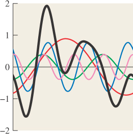
Figure 18.1: Summing up periodic functions (in color) of different frequencies leads to more complicated functions, in this case the black (thickest) one.
The same idea works for functions on the real line: We can take a function f : R ![]() R and compute (with a lot of integration) a different function
R and compute (with a lot of integration) a different function ![]() : R
: R ![]() R with the property that
R with the property that ![]() (ω) tells us “how much f looks like a cosine of frequency ω,” just as the x-coordinate of a vector v in R3 tells us how much v “looks like” the unit vector along the x-axis. And if you tell me
(ω) tells us “how much f looks like a cosine of frequency ω,” just as the x-coordinate of a vector v in R3 tells us how much v “looks like” the unit vector along the x-axis. And if you tell me ![]() , I can recover f from it. So the f ⇔
, I can recover f from it. So the f ⇔ ![]() correspondence gives us two different ways to look at any function: The first (“the value representation”) tells the value of a function at each point; the second (“the frequency representation”) tells “how much it looks like a periodic function of frequency ω” for any ω.
correspondence gives us two different ways to look at any function: The first (“the value representation”) tells the value of a function at each point; the second (“the frequency representation”) tells “how much it looks like a periodic function of frequency ω” for any ω.
In the course of ray tracing, using one ray per pixel, traced from the pixel center, we’re taking the function S, defined on R, and evaluating it at the pixel centers, which we’ll assume are the integer points; that is, we’re looking at S(0), S(1), S(2), etc. It’s quite possible for two different functions S and T to have the same integer samples (see Figure 18.2). That’s reason for concern: The samples we’re collecting don’t uniquely determine the arriving light! Even so, when we display those samples on a (one-dimensional) LCD screen, we get a piecewise constant function (see Figure 18.3) that’s not very different from either S or T. And anyhow, our eyes tend to smooth out the transitions between adjacent display pixels, making the approximation even better.
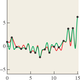
Figure 18.2: The functions S (red) and T (green) have the same values at each integer point (black dots).
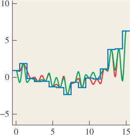
Figure 18.3: The light resulting from displaying samples of either the red or the green function on a 1D LCD screen, plotted in blue.
How serious a problem is the nonuniqueness of the preceding paragraph? Very. It’s what makes sloping straight lines on a black-and-white display look jagged, what makes wagon wheels appear to rotate backward in old movies, what makes scaled-down images look bad, and a whole host of other problems. It’s got a name: aliasing. We’ll now see where that name came from by looking at the samples of some very simple functions: the periodic functions from which all other functions can be created.
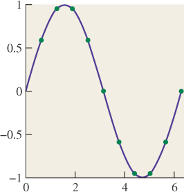
Let’s look at the interval [0, 2π], and consider ten equally spaced samples of the function x ![]() sin(x) on this interval, shown in Figure 18.4. From these samples, it’s pretty easy to reconstruct the original sine function. We can come very close to reconstructing it by just “connecting the dots,” for instance.
sin(x) on this interval, shown in Figure 18.4. From these samples, it’s pretty easy to reconstruct the original sine function. We can come very close to reconstructing it by just “connecting the dots,” for instance.
The same thing is true for the samples of x ![]() sin(2x) or (barely) x
sin(2x) or (barely) x ![]() sin(3x). But by the time we look at x
sin(3x). But by the time we look at x ![]() sin(5x) (see Figure 18.5), something odd happens: The samples are all zeroes. By looking at only the samples, we can’t tell the difference between sin(5x) and sin(0x). As Figure 18.6 shows, the same is true for sin(1x) and sin(11x).
sin(5x) (see Figure 18.5), something odd happens: The samples are all zeroes. By looking at only the samples, we can’t tell the difference between sin(5x) and sin(0x). As Figure 18.6 shows, the same is true for sin(1x) and sin(11x).
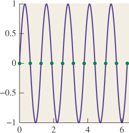

The means that if our arriving-light function S happened to be x ![]() sin(11x), we might think, from looking at the recorded samples, that it was sin(x) instead: The frequency-11 sine is masquerading as a frequency-1 sinusoid. It’s the fact that the sample values correspond to various different sinusoids that leads to the name “aliasing.” In general, if we take 2N equispaced samples, then sines of frequency k and k + 2N and k + 4N, etc., will all have identical samples. But if we restrict our function S to contain only frequencies strictly between –N and N, then the samples uniquely determine the function. The same idea works for functions defined on R rather than on an interval: If
sin(11x), we might think, from looking at the recorded samples, that it was sin(x) instead: The frequency-11 sine is masquerading as a frequency-1 sinusoid. It’s the fact that the sample values correspond to various different sinusoids that leads to the name “aliasing.” In general, if we take 2N equispaced samples, then sines of frequency k and k + 2N and k + 4N, etc., will all have identical samples. But if we restrict our function S to contain only frequencies strictly between –N and N, then the samples uniquely determine the function. The same idea works for functions defined on R rather than on an interval: If ![]() (ω) = 0 for ω ≥ ω0, then f can be reconstructed from its values at any infinite sequence of points with spacing π/ω0.
(ω) = 0 for ω ≥ ω0, then f can be reconstructed from its values at any infinite sequence of points with spacing π/ω0.
We can’t actually constrain the arriving-light function to not have high frequencies, however. If we photograph a picket fence from far away, the bright pickets against the dark grass can occur with arbitrarily high frequencies. The shorthand description of this situation is that “If your scene has high frequencies in it, then you’ll get aliasing when you render it.” The solution is to apply various tricks to remove the high frequencies before we take the samples (or in the course of sampling). Doing so in a way that’s computationally efficient and yet effective requires the deeper understanding that the rest of this chapter will give you.
Here’s one example of a trick to remove high frequencies, just to give you a taste. Consider the sin(x) versus sin(11x) example we looked at earlier. We sampled these two functions at certain values of x. Let’s say one of them is x0. What would happen if you took your input signal S and instead of computing S(x0), you computed ![]() (S(x0) + S(x0 + r1) + S(x0 – r2)), where r1 and r2 are small random numbers, on the order of half the sample spacing of 2π/10? If the input signal S were S(x) = sin(x), the three values you’d average would all be very close to sin(x0); that is, the randomization would have little effect (see Figure 18.7). On the other hand, if the original signal was S(x) = sin(11x), then the three values you’d average would tend to be very different, and their average (see Figure 18.8) would generally be closer to zero than S(x0). In short, this method tends to attenuate high-frequency parts of the input, while retaining low-frequency parts.
(S(x0) + S(x0 + r1) + S(x0 – r2)), where r1 and r2 are small random numbers, on the order of half the sample spacing of 2π/10? If the input signal S were S(x) = sin(x), the three values you’d average would all be very close to sin(x0); that is, the randomization would have little effect (see Figure 18.7). On the other hand, if the original signal was S(x) = sin(11x), then the three values you’d average would tend to be very different, and their average (see Figure 18.8) would generally be closer to zero than S(x0). In short, this method tends to attenuate high-frequency parts of the input, while retaining low-frequency parts.
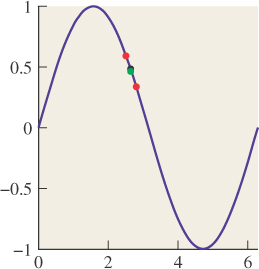
Figure 18.7: The original sample sin(x0) in black, with two nearby random samples, shown in red. The average (green) of the three heights is very nearly sin(x0).
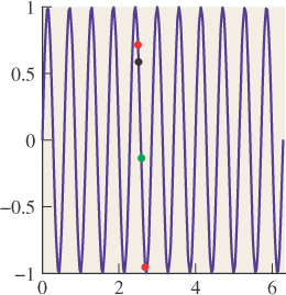
Figure 18.8: Random samples (red) of x ![]() sin(11x) near x = x0 are quite different from the sample at x0 (black), so their average (green) is nearer to zero.
sin(11x) near x = x0 are quite different from the sample at x0 (black), so their average (green) is nearer to zero.
18.1.2. Important Terms, Assumptions, and Notation
The main ideas we’ll use in this chapter are convolution and the Fourier transform, which you may have encountered in algorithms courses or in the study of various engineering or mathematics problems.
Fortunately, both convolution and Fourier transforms can be well understood in terms of familiar operations in graphics; we motivate the mathematics by showing its connection to graphics. Convolution, for instance, takes place in digital cameras, scanners, and displays. The Fourier transform may be less familiar, although the typical “graphical display” of an audio signal (see Figure 18.9), in which the amounts of bass, midrange, and treble are shown changing over time, shows, at each time, a kind of basic Fourier transform of a brief segment of the audio signal.

For us, the essential property of the Fourier transform is that it turns convolution of functions, which is somewhat messy, into multiplication of other functions, which is easy to understand and visualize.
The Fourier transformation (for functions on the real line) takes a function and represents it in a new basis; thus, this chapter provides yet another instance of the principle that expressing things in the right basis makes them easy to understand.
The same tools we use to understand images in this chapter will prove useful not only in analyzing image operations, however: They also appear in the study of the scattering of light by a surface, which can be interpreted as a kind of convolution operation [RH04], and in rendering, in which the frequency analysis of light being transported in a scene can yield insights into the nature of computations necessary to accurately simulate that light transport [DHS+05].
Before discussing convolution and other operations, we return to the topic of Section 9.4.2: the principle that you must know the meaning of every number in a graphics program. Before we discuss operations like convolution and Fourier transforms on images, we have to know what the images mean. The difficulty, which we discussed briefly in Chapter 17, is that in some cases we just don’t know. Alvy Ray Smith made a point of this in a paper titled “A Pixel Is Not A Little Square” [Smi95], in which he observes that the individual values in a pixel array do not in general represent the average of something over a small square on the image plane, and that algorithms that rely on this model of pixels are bound to fail in some cases. (More simply, he points out that a pixel does not represent a tiny square of constant value, even though the pixel may be displayed that way on an LCD screen!) As an extreme example, an object ID image contains, at each pixel, an identifier that tells which object is visible at that pixel. The pixel values in this case are not even necessarily numerical!
For this chapter only, to avoid messiness introduced by shifting by one-half in the x- and y-directions, we’re going to use display screen coordinates in which the display pixel indexed by (0, 0) has display coordinates that range from – ![]() to
to ![]() in both x and y, and the display pixel named (i, j) is a small square centered at (i, j) rather than at (i +
in both x and y, and the display pixel named (i, j) is a small square centered at (i, j) rather than at (i + ![]() , j +
, j + ![]() ). This means that pixel (i, j) is at x-location i and y-location j, and not in “row i and column j”; that is, we’re using geometric indexing rather than image indexing. Because this chapter contains no actual algorithms that depend on display pixel coordinates, this should cause no problems for you.
). This means that pixel (i, j) is at x-location i and y-location j, and not in “row i and column j”; that is, we’re using geometric indexing rather than image indexing. Because this chapter contains no actual algorithms that depend on display pixel coordinates, this should cause no problems for you.
For this chapter, we’re going to assume (initially) that images contain physical measurements of light, measured in physical units. For a digital camera, this might be something like the average radiance along a ray hitting a small rectangle on a CCD sensor, or perhaps an integral of that radiance over the area of that rectangle, or the total light energy that arrived at the rectangle while the shutter was open. (Some digital cameras will let you get such information when you store a photo in “raw” mode, and will even tell you when the sensor was oversaturated so that the stored value is a false measurement.) For a rendered image, the value stored at a pixel might be the radiance along a ray that passed through the single point at the center of the image area corresponding to the pixel, or an average of radiances of several rays through the pixel, etc. It might even be an average of samples from a region around the pixel center, where the regions for adjacent pixel centers overlap.
18.2. Historical Motivation
When graphics researchers first wanted to draw a line on a rectangular grid of pixels, the most obvious thing to do was to write the line in the form y = mx + b, and for each integer x-value, compute y = mx + b, which was usually not an integer, round it off to an integer y′, and put a mark at location (x, y′). This only works well if m is between –1 and 1; for greater slopes, it worked better to write x = my + b, that is, to swap the roles of x and y, but that’s not germane to this discussion. The kind of line produced with this method is shown in Figure 18.10, where we’ve drawn the line using little squares as pixel marks.
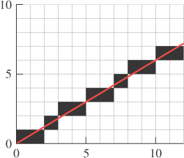
You can see that the line is fairly “jaggy”—it has jagged edges—but it’s hard to imagine how to avoid this if your only choice is to draw a black or a white square. Fortunately, display devices improved to display multiple gray levels. To avoid the staircase-like appearance of the jaggy line, we can fill in gray squares at the steps, or be even more sophisticated—we can set the gray-level for each square to be proportional to the amount that square overlaps a unit-width line, as shown in Figure 18.11. The resultant line, viewed close up like this, looks a bit odd. But seen from an appropriate distance (as in Figure 18.12), it looks very good—far better than the jaggy black-and-white line.

The “compute the overlap between the square and the thing you’re rendering” approach seems a bit ad hoc, but it also seems to work well in practice. The same idea, applied to text, produces fonts that are visually more appealing than the pure black-and-white fonts that arise when we use the “this pixel is black if the pixel center is within the character” approach (see Figures 18.13 and 18.14).


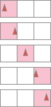
Merely computing overlaps with pixel squares isn’t a cure-all, as you can see by considering a sequence of images generated by a small moving object. Figure 18.15 shows a red triangle moving through three pixels of a “one-dimensional image” in the course of five “frames.” In the first and second frames, it’s completely in the first square, tinting it pink; in the fourth and fifth, it’s completely in the third. In frame three, it’s in the middle square. The result is that although the object is moving with uniform speed through the pixels, it appears to “rush” through the middle pixel, which is pink for only half as long as the pixels on either side.
To compensate for the differing amounts of time spent in each square, and thus the irregularity of the apparent motion, we can use a different strategy: Instead of measuring the area of the overlap between the object and the square, we can compute a weighted area overlap, counting area overlap near the square’s center as more important than area overlap near the edge of the square. While this approach does address the irregularity of the pure area-measuring approach, there remains another problem: As a small, dark object moves from left to right, the total brightness of the image varies. When the object is near the dividing line between two squares, neither is darkened much at all; when it’s near the middle of a square, that square is darkened substantially. The result is that the object appears to waver in brightness during the animation.
The somewhat surprising solution is to use a weighting function that says that an object contributes to the brightness of square i if it overlaps anywhere from the center of square i – 1 to the center of square i + 1. Figure 18.16 shows this in a side view. The object, shown as a small, black line segment, contributes both the left pixel, whose weighting function is shown in blue, and the center pixel, whose weighting function is shown in red, but not the right pixel, whose weighting function is shown in green. The left-pixel contribution is small, because the black line is near the edge of the “tent,” while the center-pixel contribution is larger. Notice that the sum of the weighting functions is the constant function 1, so no matter where we place the object, its total contribution to image brightness will be the same.
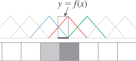
Figure 18.16: Weighted area measurement. The central red “tent-shaped” function is used as a weight for contributions to the center pixel.
We can express the weighted-area-overlap approach to determining pixel values mathematically. Let’s suppose that x ![]() f(x) is the function shown in Figure 18.16 whose value is 1 for any point x within our object, and 0 elsewhere. And let’s suppose that the red tent-shaped function in Figure 18.16 is called x
f(x) is the function shown in Figure 18.16 whose value is 1 for any point x within our object, and 0 elsewhere. And let’s suppose that the red tent-shaped function in Figure 18.16 is called x ![]() g(x). Then the value we assign to the center pixel is given by
g(x). Then the value we assign to the center pixel is given by
The value assigned to the next pixel to the right, whose weighting function is just g shifted right one unit, is
A similar expression holds for every pixel: The values we’re computing are generated by multiplying f with a shifted version of g and then integrating. This operation—point-by-point multiplication of one function by a shifted version of another, followed by integration (or summation, in some cases)—appears over and over again in both graphics and mathematics and is called convolution, although we should warn you that the proper definition includes a negation so that we end up summing things of the form f(x)h(i – x); this negation leads both to convenient mathematical properties and to considerable confusion. Fortunately for us, in almost all our applications the functions that we convolve against have the property that h(x) = h(–x), so the negative sign has no impact.
In the next section, we’ll discuss various kinds of convolutions, their applications in graphics, and some of their mathematical properties.
The remainder of this chapter consists of applying ideas from signal processing to computer graphics. In that context, functions on the real line (or an interval) are often called signals (particularly when the parameter is denoted t so that we can think of f(t) as a value that varies with time). Convolving with a function like the “tent function” above, which is nonzero on just a small region, is called applying a filter or filtering, although the term can be used for convolution with any function.
18.3. Convolution
As we said already, convolution appears over and over again in graphics and the physical world. Nearly every act of “sensing” involves some sort of convolution, for instance. For example, consider one row of sensor pixels in an idealized digital camera. We’ll say that the light energy falling on the sensor at location (x, y) in one second is described as function S(x, y), and that S is independent of time. The camera shutter opens for one second, and each pixel accumulates arriving energy over that period of time, after which an accumulated value is recorded as the pixel’s value. But each pixel sensor—say, the one at pixel (0, 0)—has a responsivity function, (x, y) ![]() M(x, y), that tells how much pixel response there is for each bit of arriving light (see Figure 18.17). We’re being deliberately informal about units here because it’s the form of the computation we care about, not the actual values.
M(x, y), that tells how much pixel response there is for each bit of arriving light (see Figure 18.17). We’re being deliberately informal about units here because it’s the form of the computation we care about, not the actual values.
To determine the sensor pixel’s response to the incoming light, we multiply each bit of light S(x, y) by the responsivity M(x, y), and sum up over the entire pixel:
If we extend the definition of M to the whole plane of the sensor by defining M to be 0 outside the unit square corresponding to pixel (0, 0), we can rewrite this as
which may appear more complicated, but actually will result in simpler formulas elsewhere.
In a well-designed camera, the sensor responsivity should be the same for each pixel. What does this mean mathematically? It means, for instance, that for sensor pixel (2, 3), we’ll want to multiply S(x, y)M(x – 2, y – 3) and integrate, that is,
and in general, the formula for sensor pixel (i, j) will be
This expression has the form of a product of a function S with a shifted function M, integrated; the resultant value is a function of the shift amount, (i, j). That is the essence of a convolution, and indeed, Equation 18.6 is almost the definition of the convolution S ![]() M of the two functions. Two small adjustments are needed. First, since S and M are both functions on all of R2, their convolution is defined to be a function on all of R2. The values we’ve described above are the restriction of that function to the integer grid. Second, it’s very convenient to have a definition of convolution that makes f
M of the two functions. Two small adjustments are needed. First, since S and M are both functions on all of R2, their convolution is defined to be a function on all of R2. The values we’ve described above are the restriction of that function to the integer grid. Second, it’s very convenient to have a definition of convolution that makes f ![]() g = g
g = g ![]() f. For this to work out properly, there needs to be an extra negation; that is, we want Equation 18.6 to have the form
f. For this to work out properly, there needs to be an extra negation; that is, we want Equation 18.6 to have the form
We can arrange this by defining ![]() (x, y) = M(–x, –y). (For a typical sensor, the response function is symmetric, so
(x, y) = M(–x, –y). (For a typical sensor, the response function is symmetric, so ![]() and M are the same.) This final form is just a 2D analog of the 1D convolution. Simplifying to one dimension, we can now define the convolution of two functions f, g : R
and M are the same.) This final form is just a 2D analog of the 1D convolution. Simplifying to one dimension, we can now define the convolution of two functions f, g : R ![]() R:
R:
(a) Pause briefly and examine that definition carefully. It’s central to much of the remainder of this book.
(b) Perform the substitution s = t–x, ds = –dx in the integral of Equation 18.8 to confirm that (f ![]() g)(t) = (g
g)(t) = (g ![]() f)(t).
f)(t).
We can say that image capture by our digital camera consists of convolving the incoming light with the “flipped” sensor response function ![]() , and then restricting to the integer lattice Z × Z.
, and then restricting to the integer lattice Z × Z.
In almost all cases that we study, one of the functions f or g will be an even function, and hence the negation has no consequence at all. The two-dimensional convolution is defined very similarly. If f, g : R2 ![]() R are two functions on R2, then
R are two functions on R2, then
Convolution is also defined for two periodic functions of period P, but with the domain of integration replaced by any interval of length P.
Convolution can also be applied to discrete signals, that is, to a pair of functions f, g : Z ![]() R; the definition is almost identical, except for the replacement of the integral with a summation:
R; the definition is almost identical, except for the replacement of the integral with a summation:
with an analogous definition for functions of two variables. If f, g : Z × Z ![]() R, then
R, then

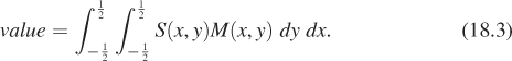
As an application of this kind of convolution, imagine that you have an image that is in very sharp focus, but you want to use it as a background for a composition in which it should appear out of focus, while the foreground objects should be in focus. One way to do this is to replace each pixel with an average of itself and its eight neighbors. Figure 18.18 shows the results on a small example. On a larger image, you might want to “blur” with a much larger block of ones, to achieve any noticeable effect. If we call f(i, j) the value of the original image pixel at (i, j), and let g(i, j) = 1 for –1 ≤ i, j ≤ 1, and 0 otherwise, then the blurred-image pixel at (i, j) is exactly (f ![]() g)(i, j). Notice, too, that the function g that we used in the blurring has the property that g(i, j) = g(–i, –j), that is, it’s symmetric about the origin, hence the negative sign in the definition of convolution is of no consequence.
g)(i, j). Notice, too, that the function g that we used in the blurring has the property that g(i, j) = g(–i, –j), that is, it’s symmetric about the origin, hence the negative sign in the definition of convolution is of no consequence.
The process we’ve just described is usually called filtering f with the filter g, where the function that’s nonzero only on a small region is called the “filter.” Because convolution is symmetric, the roles can be reversed, however, and we’ll have occasion to convolve with “filters” that are nonzero arbitrarily far out on the real line or the integers.
Consider convolving a grayscale image f with a filter g that’s defined by g(–1, –1) = g(–1, 0) = g(–1, 1) = –1, g(1, –1) = g(1, 0) = g(1, 1) = 1, and g(i, j) = 0 otherwise.
(a) Draw a plot of g.
(b) Describe intuitively where f ![]() g will be negative, positive, and zero. You might want to start out with some simple examples for f, like an all-gray image, or an image that’s white on its bottom half and black on the top, or white on the left half and black on the right, etc. Then generalize.
g will be negative, positive, and zero. You might want to start out with some simple examples for f, like an all-gray image, or an image that’s white on its bottom half and black on the top, or white on the left half and black on the right, etc. Then generalize.
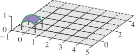
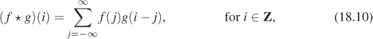
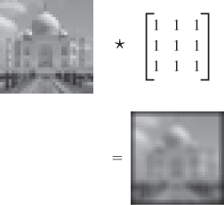
We’ve defined convolution for two continuum functions (i.e., functions defined on R) and for two discrete functions (i.e., defined on Z). There’s a third class of convolution that comes up in graphics: the discrete-continuum convolution. A familiar instance of this is display on a grayscale LCD monitor. Recall that for this chapter, the display pixel (i, j) is a small box centered at (i, j). Figure 18.19 shows the result of displaying a 2 × 2 image f (shown as a stem plot) with a “box” function b defined on R2 to produce a piecewise constant function on R2 representing emitted light intensity.
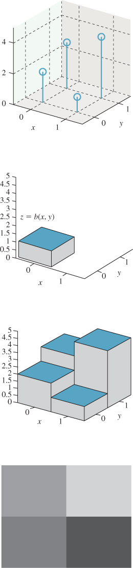
Figure 18.19: The values in a 2 × 2 grayscale image are convolved with a box function to get a piecewise constant function on a 2 × 2 square.
The emitted light at location (x, y) is given by
This doesn’t quite look like a convolution, because there’s no summation. But we can insert the summation without changing anything:
There’s no change because the box function is zero outside the unit box. In the early days of graphics, when CRT displays were common, turning on a single pixel didn’t produce a little square of light, it produced a bright spot of light whose intensity faded off gradually with distance. That meant that turning on pixel (4, 7) might cause a tiny bit of light to appear even at the area of the display we’d normally associate with coordinates (12, 23), for instance, or anywhere else. In that case, the summation in the formula for the light at position (x, y) was essential.
The general definition for the convolution of a discrete function f : Z ![]() R and a continuum function g : R
R and a continuum function g : R ![]() R is
R is

The result is a continuum function. We leave it to you to define continuous-discrete convolution, and to extend both definitions to the plane.
18.4. Properties of Convolution
As mentioned in Section 18.2, convolution has several nice mathematical properties. First, for all forms of convolution (discrete, continuous, or mixed) it’s linear in each factor, that is,
Second, it’s commutative, which we’ll show for the continuous case, answering the inline problem above:
Substituting s = t – x, ds = –dx, and x = t – s, we get
The proofs for the discrete and mixed cases are very similar.
Third, convolution is associative. The proof, which we omit, involves multiple substitutions.
Finally, continuous-continuous convolution has some special properties involving derivatives, such as f′ ![]() g = f
g = f ![]() g′ (under some fairly weak assumptions). It also generally increases smoothness: If f is continuous and g is piecewise continuous, then f
g′ (under some fairly weak assumptions). It also generally increases smoothness: If f is continuous and g is piecewise continuous, then f ![]() g is differentiable; similarly, if f is once differentiable, then f
g is differentiable; similarly, if f is once differentiable, then f ![]() g is twice differentiable. In general, if f is p-times differentiable and g is k-times differentiable, then f
g is twice differentiable. In general, if f is p-times differentiable and g is k-times differentiable, then f ![]() g is (p + k + 1)-times differentiable (again under some fairly weak assumptions).
g is (p + k + 1)-times differentiable (again under some fairly weak assumptions).
Alas, for a fixed function f, the map g ![]() f
f ![]() g is usually not invertible—you can’t usually “unconvolve.” We’ll see why when we examine the Fourier transform shortly.
g is usually not invertible—you can’t usually “unconvolve.” We’ll see why when we examine the Fourier transform shortly.
18.5. Convolution-like Computations
Convolution appears in other places as well. Consider the multiplication of 1231 by 1111:
1231
x1111
-----
1231
1231
1231
1231
-------
1367641
In computing this product, we’re taking four shifted copies of the number 1231, each multiplied by a different 1 from the second factor, summing them; this is essentially a convolution operation.
As another example, consider how a square occluder, held above a flat table, casts a shadow when illuminated by a round light source (see Figure 18.20). The brightness at a point P is determined by how much of the light source is visible from P. We can think of this by imagining the square is lit from each single point of the light source, casting a hard shadow on the surface, a shadow whose appearance is essentially a translated copy of the function f that’s one for points in the square and zero elsewhere (see Figure 18.21). We sum up these infinitely many hard-shadow pictures, with the result being a soft shadow cast by the lamp. This has the form of a convolution (a sum of many displaced copies of the same function). We can also consider the dual: Imagine each tiny bit of the rectangle individually obstructing the lamp’s light from reaching the table. The occlusion due to each tiny bit of rectangle is a disk of “reduced light”; when we sum up all these circular reductions, some table points are in all of them (the umbra), some table points are in just a few of the disks (the penumbra), and the remainder, the fully lit points, are visible to every point of the lamp. These two ways of considering the illumination arriving at the table—multiple displaced rectangles summed up, or multiple displaced disks summed up—correspond to thinking of f ![]() g as many displaced copies of f, weighted by values of g, or as many displaced copies of g, weighted by values of f.
g as many displaced copies of f, weighted by values of g, or as many displaced copies of g, weighted by values of f.

Figure 18.20: The square occluder casts a shadow with both umbra and penumbra when illuminated by a round light source.
Figure 18.21: The square shadows cast by the occluder when it’s illuminated from two different points of the light source (image lightened to better show shadows).
18.6. Reconstruction
Reconstruction is the process of recovering a signal, or an approximation of it, from its samples. If you examine Figure 18.4, for instance, you can see that by connecting the red dots, we could produce a pretty good approximation of the original blue curve. This is called piecewise linear reconstruction and it works well for signals that don’t contain lots of high frequencies, as we’ll see shortly.
We discussed earlier how the conversion of the light arriving at every point of a camera sensor into a discrete set of pixel values is modeled by a convolution, and how, if we display the image on an LCD screen, setting each LCD pixel’s brightness to the value stored in the image, we’re performing a discrete-continuous convolution, the discrete factor being the image and the continuous factor being a function that’s 1 at every point of a unit-width box centered on (0, 0) and 0 everywhere else. This second discrete-continuous convolution is another example of reconstruction, sometimes called sample and hold reconstruction.
The “take a photo, then display it on a screen” sequence (i.e., the sample-and-reconstruct sequence) is thus described by a sequence of convolutions. If taking a photo and displaying were completely “faithful,” the displayed intensity at each point would be exactly the same as the arriving intensity at the corresponding point of the sensor. But since the displayed intensity is piecewise constant, the only time this can happen is when the original lightfield is also piecewise constant (if, for instance, we were photographing a chessboard so that each square of the chessboard exactly matched one sensor pixel). In general, however, there’s no hope that sense-then-redisplay will ever produce the exact same pattern of light that arrived at the sensor. The best we can hope for is that the displayed lightfield is a reasonable approximation of the original. Since displays have limited dynamic range, however, there are practical limitations: You cannot display a photo of the sun and expect the displayed result to burn your retina.
18.7. Function Classes
There are several kinds of functions we’ll need to discuss in the next few sections. The first is the one used to mathematically model things like light arriving at an image plane, which is a continuous function of position. We can treat such a function as defined only on the image rectangle, R, or as being defined on the whole plane (which we’ll treat as R2). In either case, we require that the integral of the square of f is finite,1 that is,
1. Later we’ll consider complex-valued functions rather than real-valued ones. When we do so, we have to replace f(x) with | f(x)| in the integral.
where D is the domain on which the function is defined. (Functions satisfying this inequality are called square integrable; the interpretation, for many physically meaningful functions, is that they represent signals of finite total energy.) The domain D might be the rectangle R, the whole plane R2, the real line R, or some interval [a, b] when we’re discussing the one-dimensional situation. Functions that are square integrable form a vector space called L2, where we often write something like L2(R2) to indicate square-integrable functions on the plane. We say “f is L2” as shorthand for “f is square integrable.” The set of L2 functions on any particular domain is generally a vector space. It takes a little work to show that L2 is closed under addition, that is if f and g are L2, then so is f + g; but we’ll omit the proof, since it’s not particularly instructive.
A function x ![]() f(x) in L2(R) must “fall off” as x
f(x) in L2(R) must “fall off” as x ![]() ±∞, because if |f(x)| is always greater than some constant M > 0, then
±∞, because if |f(x)| is always greater than some constant M > 0, then ![]() , which goes to infinity as K
, which goes to infinity as K ![]() ∞.
∞.
The next class of functions is the discrete analog of L2: the set of all functions f : Z ![]() R such that
R such that
is denoted ![]() 2; these are called square summable.
2; these are called square summable.
There are two ways in which ![]() 2 functions arise. The first is through sampling of L2 functions. Sampling is formally defined in the next section, but for now note that if f is a continuous L2 function on R, then the samples of f are just the values f (i) where i is an integer, so sampling in this case amounts to restricting the domain from R to Z. The second way that
2 functions arise. The first is through sampling of L2 functions. Sampling is formally defined in the next section, but for now note that if f is a continuous L2 function on R, then the samples of f are just the values f (i) where i is an integer, so sampling in this case amounts to restricting the domain from R to Z. The second way that ![]() 2 functions arise is as the Fourier transform of functions in L2([a, b]) for an interval [a, b], which we’ll describe presently.
2 functions arise is as the Fourier transform of functions in L2([a, b]) for an interval [a, b], which we’ll describe presently.
Finally, both ![]() 2 and L2 have inner products. For
2 and L2 have inner products. For ![]() 2(Z) we define
2(Z) we define
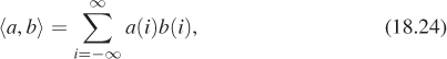
which is analogous to the definition in R3 of ![]() .
.
For L2(D), where D is either a finite interval or the real line, we define
This inner product on L2 has all the properties you might expect: It’s linear in each factor, and ![]() f, f
f, f![]() = 0 if and only if f = 0, at least if we extend the notion of f = 0 to mean that f is zero “almost everywhere,” in the sense that if we picked a random number t in the domain of f, then with probability 1, f (t) = 0. (In general, when we talk about L2, we say that two functions are equal if they’re equal almost everywhere.)
= 0 if and only if f = 0, at least if we extend the notion of f = 0 to mean that f is zero “almost everywhere,” in the sense that if we picked a random number t in the domain of f, then with probability 1, f (t) = 0. (In general, when we talk about L2, we say that two functions are equal if they’re equal almost everywhere.)
These inner-product definitions in turn let us define a notion of “length,” by defining ![]() , for f
, for f ![]() L2, and similarly for
L2, and similarly for ![]() 2. See Exercise 18.1 for further details.
2. See Exercise 18.1 for further details.
18.8. Sampling
The term sampling is much used in graphics, with multiple meanings. Sometimes it refers to choosing multiple random points Pi (i = 1, 2, ..., n) in the domain of a function f so that we can estimate the average value of f on that domain as the average of the values f (Pi) (see Chapter 30). Sometimes (as in the previous edition of this book) it’s used to mean “generating pixel values by some kind of unweighted or weighted averaging of a function on a domain,” the discrete nature of the pixel array being the motivation for the word “sampling.” In this chapter, we’ll use it in one very specific way. If f is a continuous function on the real line, then sampling f means “restricting the domain of f to the integers,” or, more generally, to any infinite set of equally spaced points (e.g., the even integers, or all points of the form 0.3 + n/2, for n ![]() Z).
Z).
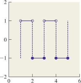
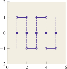
For discontinuous functions, the definition is slightly subtler; for those who’d rather ignore the details, it’s sufficient to say that if f is piecewise continuous, but has a jump discontinuity at the point x, then the sample of f at x is the average of the left and right limits of f at x. Thus, for a square wave (see Figures 18.22 and 18.23) that alternates between –1 and 1, the sample at any discontinuity is 0.
![]() The more general notion of sampling is motivated by the physical act of measurement. If we think of the variable in the function t
The more general notion of sampling is motivated by the physical act of measurement. If we think of the variable in the function t ![]() f (t) as time, then to measure f we must average its values over some nonzero period of time. If f is rapidly varying, then the shorter the period, the better the measurement. To define the sample of f at a particular time t0, we therefore mimic this measurement process. First, we consider points t0 – a and t0 + a, and define a function χt0,a : R
f (t) as time, then to measure f we must average its values over some nonzero period of time. If f is rapidly varying, then the shorter the period, the better the measurement. To define the sample of f at a particular time t0, we therefore mimic this measurement process. First, we consider points t0 – a and t0 + a, and define a function χt0,a : R ![]() R where χt0,a = 1 if t0 – a ≤ t ≤ t0 + a and 0 otherwise (see Figure 18.24). The function χt0,a serves the role of the shutter in a camera: When we multiply f by χt0,a, the values of f are “let through” only on the interval [t0 – a, t0 + a]. Next, we let
R where χt0,a = 1 if t0 – a ≤ t ≤ t0 + a and 0 otherwise (see Figure 18.24). The function χt0,a serves the role of the shutter in a camera: When we multiply f by χt0,a, the values of f are “let through” only on the interval [t0 – a, t0 + a]. Next, we let

U(a) is the “measurement” of f in the interval [t0 – a, t0 + a], in the sense that it’s the average value of f on that interval. Problem 18.2 relates this to convolution. Finally, we define the sample of f at t0 to be
that is, the limiting result of measuring f over shorter and shorter intervals. For a continuous function f, if a is small enough, then f (s) will be very close to f (t0) for any s ![]() [t0 – a, t0 + a], and the limit of U(a) is just f(t0)—the sample, defined by this measurement process, is exactly the value of f at t0 as we said above; the full proof depends on the mean value theorem for integrals. But for a discontinuous function like the square wave we saw above, the measurement process averages values to the left and right of t0, and the limit (in the case of a square wave) is the average of the upper and lower values. In cases messier than these simple ones, it can happen that the limit in Equation 18.27 can fail to exist, in which case the sample of f is not defined. We’ll never encounter such functions in practice, though.
[t0 – a, t0 + a], and the limit of U(a) is just f(t0)—the sample, defined by this measurement process, is exactly the value of f at t0 as we said above; the full proof depends on the mean value theorem for integrals. But for a discontinuous function like the square wave we saw above, the measurement process averages values to the left and right of t0, and the limit (in the case of a square wave) is the average of the upper and lower values. In cases messier than these simple ones, it can happen that the limit in Equation 18.27 can fail to exist, in which case the sample of f is not defined. We’ll never encounter such functions in practice, though.
18.9. Mathematical Considerations
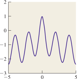
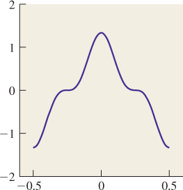
The somewhat complex definition of sampling suggests that the mathematical details of L2 functions can be quite messy. That’s true, and making precise statements about sampling, convolution, Fourier transforms, etc., is rather difficult. Often the statement of the preconditions is so elaborate that it’s quite difficult to understand what a theorem is really saying. Rather than ignoring the preconditions or precision, which leads to statements that seem like nonsense except to the very experienced, and rather than providing the exact statements of every result, we’ll restrict our attention, to the degree possible, to “nice” functions (see Figure 18.25) that are either continuous, or very nearly continuous, in the sense that they have a discrete set of discontinuities, and on either side of a discontinuity they are continuous and bounded (i.e., there’s no “asymptotic behavior” like that of the graph of y = 1/x near x = 0). Figure 18.26 shows some functions that are not nice enough to study in this informal fashion, but which also don’t arise in practice.
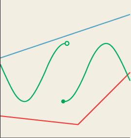
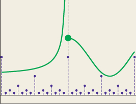
Figure 18.26: “Not-nice” functions. The blue function is 0 except at points of the form p/2q, where its value is 1/2q.
The restriction to “nice” functions is enough to make most of the subtleties disappear. It’s also appropriate in the sense that we’re using these mathematical tools to discuss physical things, like the light arriving at a sensor. At some level, that light intensity is discontinuous—either another photon arrives or it doesn’t—but at the level at which we’re hoping to model the world, it’s reasonable to treat it as a continuous function of time and position.
We’re also typically studying the result of convolving the “arriving light” function with some other function like a box; the box is a nice enough function that convolving with it always yields a continuous function, and sampling this continuous function is easy—we just evaluate at the sample points. So the way we work with light tends to mean that we’re working with functions that “behave nicely” when we look closely at the mathematics.
For the remainder of this chapter, we’ll be considering things in one dimension: Our “images” will consist of just a row of pixels; our sensor will be a line segment rather than a rectangle, etc. We’ll sometimes illustrate the corresponding ideas in two dimensions (i.e., on ordinary images), but we’ll write the mathematics in one dimension only. So we’ll be working with a function f defined on the real line, and its samples defined on the integers. To make things simpler, we’ll restrict our attention to the case where f is an even function (see Figure 18.27), where f(x) = f(–x) for every x. Examples of even functions are the cosine, and the squaring function. Restricting to even functions lets us mostly avoid using complex numbers, while losing none of the essential ideas.
To review what we’ve done so far, we’ve defined convolution, and observed that many operations like display of images, capturing images by sensing (i.e., photography or rendering), blurring or sharpening of images, etc., can be written in terms of convolution, and that sampling at a point is defined by a limit of integrals, while sampling at all points is a limit of convolutions.
For the remainder of the chapter, we’re motivated by the question, “Suppose we have incoming light arriving at a sensor, and we want to make an image that best captures this arriving light for subsequent display or other uses; what should we store in the image array?” To answer this question, we need to do two things.
• Choose a new basis in which to represent images.
• Understand how convolution “looks” in this new basis.
The Fourier transform is how we’ll transform images into the new basis. And in the new basis, convolution of functions becomes multiplication of functions, which is much easier to understand and reason about.
18.9.1. Frequency-Based Synthesis and Analysis
Consider the interval H = (–![]() ,
, ![]() ], which we’ll use throughout this chapter; the letter “H” is mnemonic for “half.” By writing a sum like
], which we’ll use throughout this chapter; the letter “H” is mnemonic for “half.” By writing a sum like
shown in Figure 18.28, we can produce an even function on that interval (i.e., one symmetric about the y-axis). In general, any sum of cosines of various integer frequencies will be an even function, because each component cosine is even. By changing how much of each frequency of cosine we mix in, we can get many different functions.
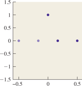
We can, for instance, find a combination of cos(0x), cos(2πx), and cos(4πx) that satisfies f(0) = 1, f(1/6) = 0, and f(![]() ) = 0. These constraints are shown in Figure 18.29; the shaded constraints on the left are there because the function is even, so its values on the left half of the real line must match those on the right half of the line.
) = 0. These constraints are shown in Figure 18.29; the shaded constraints on the left are there because the function is even, so its values on the left half of the real line must match those on the right half of the line.
We write
and then plugging in the constraints, we find that
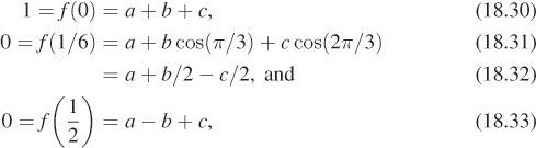
from which we can determine that a = 0 and b = c = 1/2 (see Figure 18.30).
This is easy to generalize: If we’re given k constraints on the values of a function on the non-negative part of the interval I, then we can find a function written as a linear combination of cos(0x), cos(2πx), ..., cos(2π(k – 1)x) that satisfies those constraints. The proof relies on elementary properties of the cosine and sine.
Thus, we can “synthesize” various even functions by summing up cosines of many frequencies. We can even “direct” our synthesized function to have certain values at certain points, as in the second example above. We can synthesize odd functions by summing up sines of various frequencies as well, and by mixing sines and cosines, we can even synthesize functions that are neither even nor odd. Whatever function we synthesize, however, will be periodic of period 1, because each term in the sum is periodic with that period. Thus, if f is a sum of sines and cosines of different integer frequencies, we’ll have f(![]() ) = f (–
) = f (–![]() ).
).
We’re using the term “frequency” here quite specifically: We say that x ![]() cos(2πx) is a function of frequency 1. Some other texts say that x
cos(2πx) is a function of frequency 1. Some other texts say that x ![]() cos(x) is a function of frequency 1. In the same way, some books prefer to define the Fourier transform on the interval [–1, 1], or [0, 1], or [0, 2π]; depending on the interval, this introduces a multiplicative constant in the definition of the inner product. We’re following the convention of Dym and McKean [DM85] so that the interested reader may refer there for proofs, but there is no universal standard. Fortunately for us, we’ll mostly be concerned with qualitative properties of the Fourier transform, for which the interval of definition and multiplicative constants are not important.
cos(x) is a function of frequency 1. In the same way, some books prefer to define the Fourier transform on the interval [–1, 1], or [0, 1], or [0, 2π]; depending on the interval, this introduces a multiplicative constant in the definition of the inner product. We’re following the convention of Dym and McKean [DM85] so that the interested reader may refer there for proofs, but there is no universal standard. Fortunately for us, we’ll mostly be concerned with qualitative properties of the Fourier transform, for which the interval of definition and multiplicative constants are not important.
More surprising, perhaps, is that any even continuous function f on the interval H that satisfies f(![]() ) = f(–
) = f(–![]() ) can be written as a sum of cosines of various integer frequencies. Even discontinuous functions can be almost written as such a sum. For instance, the square-wave function (see Figure 18.31) defined by
) can be written as a sum of cosines of various integer frequencies. Even discontinuous functions can be almost written as such a sum. For instance, the square-wave function (see Figure 18.31) defined by


can be almost expressed by the infinite sum

We say “almost expressed” because ![]() (±
(±![]() ) = 0—the average of the values of f to the left and right of ±
) = 0—the average of the values of f to the left and right of ±![]() —rather than being equal to f(±
—rather than being equal to f(±![]() ) = 1.
) = 1.
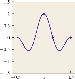
The sequence in Equation 18.35 can be approximated by taking a finite number of terms; a few of those approximations are shown in Figure 18.32.
Figure 18.32: The square wave approximated by 2, 10, and 100 terms. The slight overshoot in the approximations is called ringing.
As a more graphically oriented example, let’s take one row of pixels from a symmetric image like that shown in Figure 18.33. We’ve actually taken half a row and flipped it over to get a perfectly symmetric line of 3,144 pixels, shown in Figure 18.34.
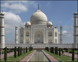
Figure 18.33: The Taj Mahal. Original image by Jbarta, at http://upload.wikimedia.org/wikipedia/commons/b/bd/Taj_Mahal,_Agra,_India_edit3.jpg.
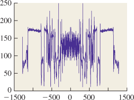
If we write this function as a sum of cosines, the sum will have 3,144 terms, which is hard to read. It starts out as
We can make an abstract picture of this summation by plotting the coefficients: At 0 we plot 129.28, at 1 we plot 5.67, at 2 we plot –2.34, etc. The result is shown in Figure 18.35, except that since the coefficient of cos(0x) is actually 141.8, we’ve adjusted the y-axis so that you can see the other details, thus hiding the large coefficient for the cos(0x) term. (That coefficient is just the average of all the pixel values.)
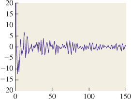
Figure 18.35: The first few coefficients for the sum representing the row of Taj Mahal pixels. We plot the coefficient of cos(2πkx) at position k.
Notice that as the frequencies get higher, the coefficients get smaller. In fact, in natural images, this “falling off with higher frequencies” is commonplace. Notice too that the function shown in Figure 18.34 has lots of variation at a very small scale, while the one shown in Figure 18.28 has variation only at a very large scale. If we made a plot for Figure 18.28 analogous to Figure 18.35, it would have only two nonzero values (at frequencies 0 and 1). In general, details at small scales mean there must be high frequencies in the image, just as we observed in Section 18.11. Since x ![]() cos(2πkx) has “features” at a scale of
cos(2πkx) has “features” at a scale of ![]() , in general any sum that stops at the cos(2πkx) term will have no features smaller than
, in general any sum that stops at the cos(2πkx) term will have no features smaller than ![]() . This kind of relationship between the pattern of coefficients and the appearance of the pixel-value plot is a powerful reasoning tool. We’ll next formalize it using the Fourier transform.
. This kind of relationship between the pattern of coefficients and the appearance of the pixel-value plot is a powerful reasoning tool. We’ll next formalize it using the Fourier transform.
But first, it’s useful to understand how the frequency decomposition of an image actually looks, so Figure 18.36 shows these to you, for a grayscale version of the Taj Mahal image (again, symmetrized). The frequency-0 part of the image is the average grayscale value; we’ve actually included this in both the middle-and high-frequency images to prevent having to use values less than 0.

18.10. The Fourier Transform: Definitions
In the next two sections we’ll define several different Fourier transforms, all of them closely related. We’ll only hint at the proofs of various claims, and instead rely mostly on suggestive examples. As motivation for you as you read these sections, here are the three main features of the Fourier transform that we’ll use in applications to computer graphics.
• The Fourier transform turns convolution into multiplication, and vice versa. If we write ![]() for the Fourier transform, this means that
for the Fourier transform, this means that
• If we define a function g like the one shown in Figure 18.37, with peaks that are equally spaced and very narrow, then the Fourier transform of g looks rather like g itself, except that the closer the spacing of the peaks in g, the wider the spacing of the peaks in the transform.

• Multiplying a function f by a function like g approximates “sampling f at equispaced points.” Thus, functions like g can be used to study the effects of sampling. Because of the convolution-multiplication duality, we’ll see that the sampled function has a Fourier transform that’s a sum of translated replicates of the original function’s transform.
18.11. The Fourier Transform of a Function on an Interval
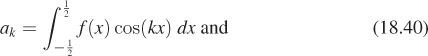
We hinted in Section 18.9.1 that if we had an even function in L2(H), then its Fourier transform was the set of coefficients used to write the function as a sum of cosines. In general, however, the Fourier transform is defined for any L2 function, not just even ones. The most basic definition is a little messy. For each integer k ≥ 0, define
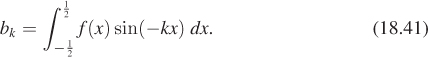
Notice that b0 is always 0.
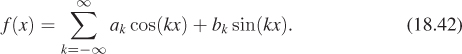
The sequences {ak} and {bk} are called the Fourier transform of f. If f is continuous and ![]() , then it turns out that
, then it turns out that
Surprisingly, the annoyance of having an unnecessary value (b0), the vagueness of “the Fourier transform consists of two sequences,” and the somewhat surprising appearance of the negative sign in the definition of bk can all be resolved by generalizing to complex numbers.
Instead of real-valued functions ![]() , we’ll consider complex-valued functions. And instead of considering the sine and cosine separately, we’ll define
, we’ll consider complex-valued functions. And instead of considering the sine and cosine separately, we’ll define
Show that (ek(x)+e–k(x))/2 = cos(2πkx), and (ek(x) – e–k(x))/(2i) = sin(2πkx), so that any function written as a sum of sines and cosines can also be written as a sum of eks, and vice versa.
The only other change is that the definition of the inner product must be slightly modified to
where ![]() is the complex conjugate. Making this change ensures that the inner product of f with f is always a non-negative real number so that its square root can be used to define the length ||f||.
is the complex conjugate. Making this change ensures that the inner product of f with f is always a non-negative real number so that its square root can be used to define the length ||f||.
With this inner product, the set of functions {ek : k ![]() Z} is orthonormal, that is,
Z} is orthonormal, that is,

the proof is an exercise in calculus and trigonometric identities.
We define
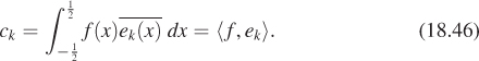
It then turns out that for a continuous L2 function f satisfying ![]() ,
,
that is, computing the inner product of f with each basis element ek lets us write f as a linear combination of the ek’s. This is exactly analogous to the situation in R3, where a vector is the sum of its projections onto the three coordinate axes. The only difference here is that the sum is infinite, and so a proof is needed to establish that it converges.
The Fourier transform of f is now defined to be the sequence {ck : k ![]() Z}. With this revised definition, we see that the Fourier transform of f is just the list of coefficients of f when it’s written in a particular orthonormal basis. Such “lists of coefficients” form a vector space under term-by-term addition and scalar multiplication, and the Fourier transform is a linear transformation from L2 to this new vector space. Be sure you understand this: The Fourier transform is just a change of representation. It’s a very important one, though, because of the multiplication-convolution property.
Z}. With this revised definition, we see that the Fourier transform of f is just the list of coefficients of f when it’s written in a particular orthonormal basis. Such “lists of coefficients” form a vector space under term-by-term addition and scalar multiplication, and the Fourier transform is a linear transformation from L2 to this new vector space. Be sure you understand this: The Fourier transform is just a change of representation. It’s a very important one, though, because of the multiplication-convolution property.
The function f ![]() L2(H) is often referred to as being in the time domain, while its Fourier transform is said to be in the frequency domain. Since one is a function on an interval and the other is a function on the integers, the distinction between the two is quite clear. But for functions in L2(R), the Fourier transform is also in L2(R), and so being able to talk about the two domains is helpful. We’ll sometimes use “value domain” or “value representation” for the original function, and “frequency representation” for its Fourier transform, because f(x) tells us the value of f at x, while ck tells us how much frequency-k content there is in f.
L2(H) is often referred to as being in the time domain, while its Fourier transform is said to be in the frequency domain. Since one is a function on an interval and the other is a function on the integers, the distinction between the two is quite clear. But for functions in L2(R), the Fourier transform is also in L2(R), and so being able to talk about the two domains is helpful. We’ll sometimes use “value domain” or “value representation” for the original function, and “frequency representation” for its Fourier transform, because f(x) tells us the value of f at x, while ck tells us how much frequency-k content there is in f.
We mostly won’t care about the particular values ck in what follows, but we’ll want to be able to take a big-picture look at these numbers and say things like “For this function, it turns out that ck = 0 whenever |k| > 200,” or “The complex numbers ck get smaller and smaller as k gets larger.” (Recall that the “size” of a complex number z = a+bi is called its modulus, and is ![]() .) Because of this big-picture interest, rather than trying to plot ck for k
.) Because of this big-picture interest, rather than trying to plot ck for k ![]() Z, we instead plot |ck|. The advantage is that |ck| is a real number rather than a complex one, so it’s easier to plot. The plot of these absolute values is called the spectrum of f, and it tells us a lot about f. (The word “spectrum” arises from a parallel with light being split into all the colors of the spectrum.)
Z, we instead plot |ck|. The advantage is that |ck| is a real number rather than a complex one, so it’s easier to plot. The plot of these absolute values is called the spectrum of f, and it tells us a lot about f. (The word “spectrum” arises from a parallel with light being split into all the colors of the spectrum.)
The Fourier transform takes a function in L2(H) and produces the sequence of coefficients ck. It’s useful to think of this sequence as a function defined on the integers, namely k ![]() ck. In fact, the sum
ck. In fact, the sum
turns out to be the same as ![]() , which is finite because f is an L2 function. This means that k
, which is finite because f is an L2 function. This means that k ![]() ck is an
ck is an ![]() 2 function, and thus the Fourier transform takes L2(H) to
2 function, and thus the Fourier transform takes L2(H) to ![]() 2(Z). From now on we’ll denote the Fourier transform with the letter
2(Z). From now on we’ll denote the Fourier transform with the letter ![]() , so
, so
Notice that ![]() (f) is a function:
(f) is a function: ![]() (f)(k) is defined to be ck, the kth Fourier coefficient for f. For simplicity, we’ll sometimes denote the Fourier transform of f by
(f)(k) is defined to be ck, the kth Fourier coefficient for f. For simplicity, we’ll sometimes denote the Fourier transform of f by ![]() .
.
We’ll often use two properties of the Fourier transform.
• First, if f is an even function, then each ck is a real number (i.e., its imaginary part is 0). For even functions, we can therefore actually plot ck rather than |ck|; that’s what we did in Figure 18.35, although we only plotted it for k ≥ 0.
• Second, if f is real-valued (as are all the functions we care about, the real value being something like “the intensity of light arriving at this point”), then its Fourier transform is even, that is, ck = c–k for every k. That’s why we showed the plot of ck for k ≥ 0 in Figure 18.35: The values for k < 0 would have added no information.
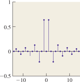
We have one example of the Fourier transform already: We wrote the square-wave function s, as a sum of cosines in Equation 18.35. From that sum, we can read off
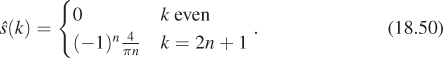
The plot of ![]() is shown in Figure 18.38.
is shown in Figure 18.38.
18.11.1. Sampling and Band Limiting in an Interval
Now suppose that we have a function f on the interval H with ![]() (f)(k) = 0 for all |k| > k0. Such a function is said to be band-limited at k0. The function f can be written as a sum of sinusoidal functions, all of frequency less than or equal to k0. Since the “features” of a sinusoidal function of frequency k (the “bumps”) are of size
(f)(k) = 0 for all |k| > k0. Such a function is said to be band-limited at k0. The function f can be written as a sum of sinusoidal functions, all of frequency less than or equal to k0. Since the “features” of a sinusoidal function of frequency k (the “bumps”) are of size ![]() , the features of f must be no smaller than
, the features of f must be no smaller than ![]() . We can say that the function f is “smooth at the scale
. We can say that the function f is “smooth at the scale ![]() .” In a technical sense, f is completely smooth, but what we mean is that f has no bumpiness smaller than
.” In a technical sense, f is completely smooth, but what we mean is that f has no bumpiness smaller than ![]() .
.
Turning this notion around, suppose that the graph of f has a sharp corner, or a discontinuity. Then f cannot be band-limited—it must be made up of sinusoids of arbitrarily high frequencies! This is important: A function that’s discontinuous, or nondifferentiable, cannot be band-limited. The converse is false, however—there are plenty of smooth functions that contain arbitrarily high frequencies.
The set of all functions band-limited at k0 is a vector space—if we add two band-limited functions, we get another band-limited function, etc. The dimension of this vector space is 2k0 + 1, with coordinates provided by the numbers c0, c±1, ..., c±k0. (This is the dimension as a real vector space; each number cj has a real and an imaginary part, contributing two dimensions, except for c0, which is pure real.)
If we evaluate the function f at k0 + 1 equally spaced points in the interval H = (–![]() ,
, ![]() ] we get k0 + 1 complex numbers, which we can treat as 2k0 + 2 real numbers. If we ignore any one of these, we’re left with 2k0 + 1 real numbers. That is to say, we’ve defined a linear mapping from the band-limited functions to R2k0+1. This mapping turns out to be bijective. (The proof involves lots of trigonometric identities and some complex arithmetic.) What that tells us is somewhat remarkable:
] we get k0 + 1 complex numbers, which we can treat as 2k0 + 2 real numbers. If we ignore any one of these, we’re left with 2k0 + 1 real numbers. That is to say, we’ve defined a linear mapping from the band-limited functions to R2k0+1. This mapping turns out to be bijective. (The proof involves lots of trigonometric identities and some complex arithmetic.) What that tells us is somewhat remarkable:
If f is band-limited at k0, then any k0 + 1 equally spaced samples of f determine f uniquely. Conversely, if you are given values for k0 + 1 equally spaced samples (except for either the real or complex part of one value), then there’s a unique function f, band-limited at k0, that takes on those values at those points.
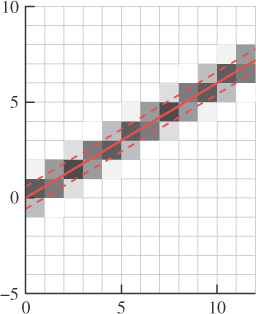
This is one form of the Shannon sampling theorem [Sha49] or simply sampling theorem. We can apply this to real-valued functions, whose Fourier transforms are even functions. This means that c–1 = c1, and c–2 = c2, etc. So, of the 2k0 + 1 degrees of freedom, we have only k0 + 1 degrees of freedom for a real-valued function. In this case, the sampling theorem says:
Suppose that f and g are real-valued functions on [–![]() ,
, ![]() ], and x0, ..., xk0 are k0 + 1 evenly spaced points in that interval, for example,
], and x0, ..., xk0 are k0 + 1 evenly spaced points in that interval, for example,
and yj = f(xj) for j = 0, ..., k0, and ![]() = g(xj).
= g(xj).
If yj = ![]() for all j, then f and g are equal, that is, a function band-limited at k0 is completely determined by k0 + 1 equally spaced samples. Furthermore, given any set of values
for all j, then f and g are equal, that is, a function band-limited at k0 is completely determined by k0 + 1 equally spaced samples. Furthermore, given any set of values ![]() , there is a unique function, f, band-limited at k0, with f(xj) = yj for every j.
, there is a unique function, f, band-limited at k0, with f(xj) = yj for every j.
Peeking ahead, this theorem is important because we generally build an image by taking equispaced samples of some function f, and we hope that the image really “captures” whatever information is in f. The sampling theorem says that if f is band-limited at some frequency, and if we take an appropriate number of samples for that frequency, then we can reconstruct f from the samples, that is, the image is a faithful representation of the function f.
This should make you ask, “Well, what happens if I take k0 samples of a real-valued function that’s not band-limited at k0? What band-limited function do those correspond to?” We’ll address this soon.
On the interval H = (–![]() ,
, ![]() ], consider the three points –
], consider the three points –![]() , 0, and
, 0, and ![]() .
.
(a) What real-valued function, f1, band-limited at k0 = 1, has values 1, 0, and 0 at these points? What functions f2 and f3 correspond to value sets 0, 1, 0 and 0, 0, 1? (You may want to use a computer algebra system to solve these parts.)
(b) Now find a band-limited function whose values at the three points are –![]() , 1, –
, 1, –![]() .
.
(c) What are the samples of x ![]() cos(4πx) at these three points? Does this contradict the sampling theorem?
cos(4πx) at these three points? Does this contradict the sampling theorem?
The sampling theorem can be read in reverse: If I’m taking samples with a spacing h between them, what’s the highest frequency I can tolerate in my signal if I want to be able to reconstruct it from the samples? The answer is that the wavelength of the signal must be greater than twice h. The frequency, known as the Nyquist frequency, is therefore π/h.
Suppose you prefer the convention that x ![]() sin(x) has frequency 1. What’s the Nyquist frequency if the sample spacing is h?
sin(x) has frequency 1. What’s the Nyquist frequency if the sample spacing is h?
18.12. Generalizations to Larger Intervals and All of R
If instead of functions on H = (–![]() ,
, ![]() ] we want to study functions on the interval (–M/2, M/2] of length M, we can make analogous definitions. The definition of the Fourier transform gets an extra factor of
] we want to study functions on the interval (–M/2, M/2] of length M, we can make analogous definitions. The definition of the Fourier transform gets an extra factor of ![]() ; the limits of integration change to ±M/2, and instead of using the function ek, for k
; the limits of integration change to ±M/2, and instead of using the function ek, for k ![]() Z, we must use
Z, we must use
The Fourier transform now sends L2(–M/2, M/2) to ![]() 2(
2(![]() Z), that is, functions on the set of all integer multiples of 1/M. Thus, as the interval we’re considering gets wider and wider (i.e., as M increases), the spacing between the frequencies involved in representing functions on that interval gets narrower and narrower.
Z), that is, functions on the set of all integer multiples of 1/M. Thus, as the interval we’re considering gets wider and wider (i.e., as M increases), the spacing between the frequencies involved in representing functions on that interval gets narrower and narrower.
It’s natural to “take a limit” and consider what happens when we let M ![]() ∞. It turns out that in addition to the Fourier transform defined for L2(–M/2, M/2), we can define a Fourier transform for L2(R).
∞. It turns out that in addition to the Fourier transform defined for L2(–M/2, M/2), we can define a Fourier transform for L2(R).
For f ![]() L2(R), we define F(f): R
L2(R), we define F(f): R ![]() R by the rule
R by the rule
where
We can think of ![]() (f)(ω) as telling “how much frequency ω stuff there is in f,” but this is a little misleading; it’s perhaps better to say that
(f)(ω) as telling “how much frequency ω stuff there is in f,” but this is a little misleading; it’s perhaps better to say that ![]() (f)(ω) says “how much f looks like a periodic function of frequency ω.”
(f)(ω) says “how much f looks like a periodic function of frequency ω.”
Just as in the case of finite intervals, if ![]() (f)(ω) = 0 for |ω| > ω0, we say that f is band-limited at frequency ω0.
(f)(ω) = 0 for |ω| > ω0, we say that f is band-limited at frequency ω0.
Before we leave the subject of Fourier transforms, there’s one last topic to cover: If we consider a periodic function h of period one, then h is definitely not in L2(R), because it doesn’t tend to zero at ±∞, so the integral of Equation 18.53 won’t generally converge. On the other hand, the corresponding integral over just one period of the function is the one used in defining the Fourier transform on an interval, Equation 18.46. Thus, we can use the interval formulation to talk about Fourier transforms for periodic functions as well.
![]() Roughly speaking, if we truncate a periodic function f of period one by setting f(x) = 0 for |x| > M, the L2(R) transform of the resultant function tends to be concentrated near integer points, and its value there tends to be proportional to M. As M gets larger, the concentration grows greater, until in the limit, the L2(R) transform is zero except at integer points, where it’s infinite. By dividing by M, at each stage we can convert the infinite values to finite ones, and they look just like the L2(H) transform of a single period of f.
Roughly speaking, if we truncate a periodic function f of period one by setting f(x) = 0 for |x| > M, the L2(R) transform of the resultant function tends to be concentrated near integer points, and its value there tends to be proportional to M. As M gets larger, the concentration grows greater, until in the limit, the L2(R) transform is zero except at integer points, where it’s infinite. By dividing by M, at each stage we can convert the infinite values to finite ones, and they look just like the L2(H) transform of a single period of f.
18.13. Examples of Fourier Transforms
18.13.1. Basic Examples
We’ve already seen (in Figures 18.34 and 18.35) the Fourier transform of one row of a natural image. The rapid falloff of ![]() (f)(ω) as ω grows is typical; in general, you can expect the Fourier transform to fall off like 1/ωa for some a > 1. For a synthetic image, which has sharp edges (e.g., a checkerboard), you might expect a 1/ω falloff, as we saw in the case of a square wave. In general, we’ll plot signals in blue and their transforms in magenta, although on a few occasions we’ll plot several signals on one axis and their transforms on another axis, using the same color for each signal and its transform. We’ll plot discrete signals—ones whose domain is Z—using stemplots.
(f)(ω) as ω grows is typical; in general, you can expect the Fourier transform to fall off like 1/ωa for some a > 1. For a synthetic image, which has sharp edges (e.g., a checkerboard), you might expect a 1/ω falloff, as we saw in the case of a square wave. In general, we’ll plot signals in blue and their transforms in magenta, although on a few occasions we’ll plot several signals on one axis and their transforms on another axis, using the same color for each signal and its transform. We’ll plot discrete signals—ones whose domain is Z—using stemplots.
18.13.2. The Transform of a Box Is a Sinc
Let
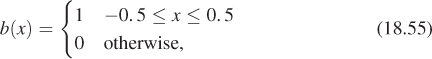
be a box function defined on the real line. Because it’s an even function and it’s real-valued, its Fourier transform will be even and real-valued. We can evaluate ![]() (b)(ω) directly from the definition.
(b)(ω) directly from the definition.


The calculation above works for all ω ≠ 0; for ω = 0, we have ![]() (b)(0) = 1, which you should verify by writing out the integral.
(b)(0) = 1, which you should verify by writing out the integral.
This computation is shown pictorially in Figure 18.39, which is adapted from Bracewell [Bra99], an excellent reference for those interested in practical signal processing.
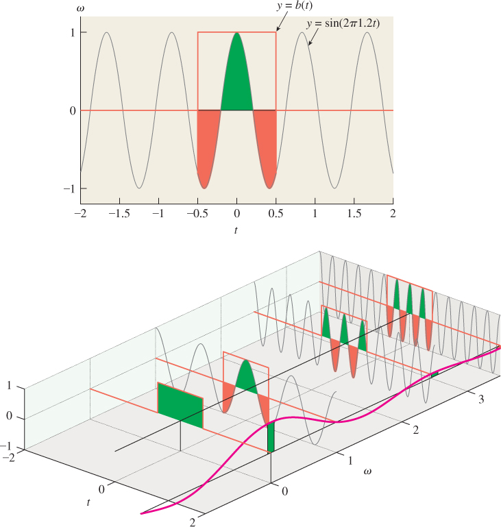
Figure 18.39: To compute the Fourier transform of the box b, for each frequency ![]() , we multiply sin(2πωx) by b and compute the area beneath the resultant function, with positive area (above the tω-plane) shown in green and negative area in red. Top: The computation for ω = 1.2. Bottom: Computations for several values of ω. For each one, we plot, at the right, the total area computed. This gives a function of the frequency ω, shown as a smooth magenta curve; the result is evidently ω
, we multiply sin(2πωx) by b and compute the area beneath the resultant function, with positive area (above the tω-plane) shown in green and negative area in red. Top: The computation for ω = 1.2. Bottom: Computations for several values of ω. For each one, we plot, at the right, the total area computed. This gives a function of the frequency ω, shown as a smooth magenta curve; the result is evidently ω ![]() sinc(ω).
sinc(ω).
Repeat the preceding computation to compute the Fourier transform of a box of width a, that is, a function that’s one on the interval [–a/2, a/2] and zero elsewhere. Hint: Substitute u = x/a in the integral to avoid doing any further work at all.
This is the only Fourier transform of a function on the real line that we’ll actually compute directly like this. The resultant function is so important that it gets its own name:
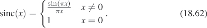
The function name is often pronounced “sink.” Despite being described by cases, the function is smooth and infinitely differentiable; its Taylor series is just the series for sin(πx) divided by πx:
18.13.3. An Example on an Interval
Consider the function f(x) = cos(2πx) (see Figure 18.40) on the interval H. Direct evaluation of the integral shows that ![]() (f)(1) =
(f)(1) = ![]() and
and ![]() (f)(–1) =
(f)(–1) = ![]() , and FT(f)(k) = 0 for all other k (see Figure 18.41). Thus, f(x) =
, and FT(f)(k) = 0 for all other k (see Figure 18.41). Thus, f(x) = ![]() e1(x) +
e1(x) + ![]() e–1(x), which is also obvious from the definition of ek(x).
e–1(x), which is also obvious from the definition of ek(x).
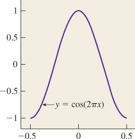
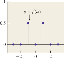
18.14. An Approximation of Sampling
If we again take a single row of the Taj Mahal signal and think of it as a function on the interval [–![]() ,
, ![]() ], we can multiply it by a function like the one shown in Figure 18.42, which removes most of the signal and retains only a small neighborhood of many evenly spaced points (we actually used a sampling function with about 100 peaks). Figure 18.43 shows the result near the center of the row, using pixel coordinates for the x-axis. As you can see, the resultant signal consists of many small peaks. This spiky signal has a Fourier transform that looks somewhat like the original Fourier transform, replicated over and over again (see Figures 18.44 and 18.45). This replication will be explained soon.
], we can multiply it by a function like the one shown in Figure 18.42, which removes most of the signal and retains only a small neighborhood of many evenly spaced points (we actually used a sampling function with about 100 peaks). Figure 18.43 shows the result near the center of the row, using pixel coordinates for the x-axis. As you can see, the resultant signal consists of many small peaks. This spiky signal has a Fourier transform that looks somewhat like the original Fourier transform, replicated over and over again (see Figures 18.44 and 18.45). This replication will be explained soon.
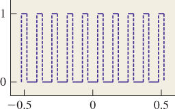
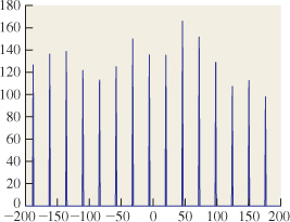
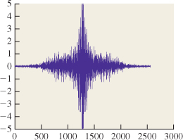
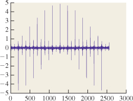
The replication in this example isn’t exact by any means. That’s partly because we’ve used “wide” peaks to do the sampling, and partly because the Taj Mahal data itself is made of samples rather than being a true function on the real line, and we didn’t do interpolation to turn it into such a function. But if the Taj data were a continuous function defined on the interval, and if our sampling peaks were very narrow, the Fourier transform would consist of a sum of almost exact replicates of the transform of the unsampled image.
You’ll also notice that the transform of the sampled image isn’t as large (on the y-axis) as the original (look carefully at the labels on the y-axis). That’s because in our “sampling” process we’ve removed a lot of the data and replaced it with zeroes, hence every integral tends to get smaller.
18.15. Examples Involving Limits
We need two more examples, each of which involves not a single function but a sequence of functions.
18.15.1. Narrow Boxes and the Delta Function
As you found when you computed the transform for a box of width a, as the box grows narrower, the transform grows wider: It’s sinc-like, but instead of having zeroes at integer points, it has zeroes at multiples of 1/a. You may also have noticed that, just as with the sampled Taj Mahal data, it gets smaller in the vertical direction: While the transform of the unit-width box reached height 1 (at ω = 0), the transform of a box of width a reaches height a at ω = 0.
Let’s consider now
which for any nonzero a is a box of width a and height 1/a so that the area under the box is always 1. Figure 18.46 shows a few examples. For any a, the transform of x ![]() g(x, a) is a sinc-like function with value 1 at ω = 0, but as a
g(x, a) is a sinc-like function with value 1 at ω = 0, but as a ![]() 0, the “width” of the sinc grows greater and greater. Figure 18.47 shows the results.
0, the “width” of the sinc grows greater and greater. Figure 18.47 shows the results.
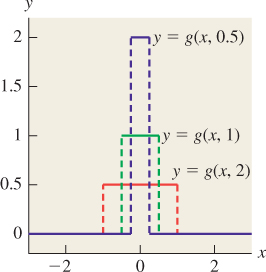
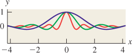
The sequence of functions x ![]() g(x, a), as a
g(x, a), as a ![]() 0, produces a sequence of Fourier transforms that approaches the constant function ω
0, produces a sequence of Fourier transforms that approaches the constant function ω ![]() 1. In many engineering textbooks, the “limit” of this sequence is defined to be “the delta function x
1. In many engineering textbooks, the “limit” of this sequence is defined to be “the delta function x ![]() δ(x),” and its Fourier transform is observed to be the constant function 1. This literally makes no sense: The sequence of functions does not approach a limit at x = 0, and the supposed Fourier transform is not in L2, because the integral of its square is not finite. Nonetheless, with some care one can work with the delta function by constantly remembering that the ordinary rules don’t actually apply to it, and it’s really a proxy for a limiting process.
δ(x),” and its Fourier transform is observed to be the constant function 1. This literally makes no sense: The sequence of functions does not approach a limit at x = 0, and the supposed Fourier transform is not in L2, because the integral of its square is not finite. Nonetheless, with some care one can work with the delta function by constantly remembering that the ordinary rules don’t actually apply to it, and it’s really a proxy for a limiting process.
![]() The only way in which we’ll ever want to use the δ function, or the comb function defined in the next section, is inside a mapping like
The only way in which we’ll ever want to use the δ function, or the comb function defined in the next section, is inside a mapping like
that is, to define a real-valued function on L2, which is a covector for L2. If we replace δ(x) in Equation 18.65 with g(x, a), and take a limit as a ![]() 0, the resultant sequence of covectors actually does converge, although this requires proof. Thus, the δ function, at least inside an integral, makes some sense.
0, the resultant sequence of covectors actually does converge, although this requires proof. Thus, the δ function, at least inside an integral, makes some sense.
18.15.2. The Comb Function and Its Transform
In much the same way we just analyzed a sequence of ever-narrower-and-taller box functions, we can consider a sequence of L2(R) functions that approaches a comb, a function with an “infinitely narrow box” at every integer. Figure 18.48 shows how we can do this: We place boxes of width a and height 1/a at each integer point, but then multiply their heights by a “tapering” function of width proportional to 1/a so that the total area under all the boxes is finite, hence the functions are all in L2(R).
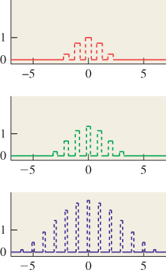
Figure 18.49 shows the transforms of these functions. Just as with the delta function, the transforms seem to approach a limit, but in this case the limit is again the comb function (i.e., the transform grows larger and larger at integer points, while heading toward zero at all noninteger points).
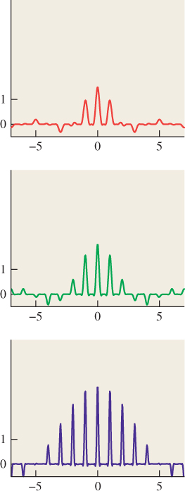
We’ll use the symbol ψ for the comb; informally, we say that ![]() (ψ) = ψ. If we create a comb with spacing c instead of 1, its transform is a comb with spacing 1/c, just as we saw with the box and the sinc.
(ψ) = ψ. If we create a comb with spacing c instead of 1, its transform is a comb with spacing 1/c, just as we saw with the box and the sinc.
18.16. The Inverse Fourier Transform
We’ve already said that if we take a function f in L2(H) (or a periodic function of period one) and compute its Fourier transform ck = ![]() (f)(k), then we can recover f by writing
(f)(k), then we can recover f by writing
For a nice function f, this sum equals f except at points of discontinuity of f, and possibly the endpoints, if f(![]() ) ≠ f(–
) ≠ f(–![]() ). Thus, we’ve defined an inverse transform that takes a sequence of coefficients and produces an L2 function on the interval (or a periodic function of period one).
). Thus, we’ve defined an inverse transform that takes a sequence of coefficients and produces an L2 function on the interval (or a periodic function of period one).
There’s a similar “inverse transform” defined for L2(R):
with the same kind of property: If we transform a nice function f to get g, and then inverse-transform g, we get back a function that’s equal to f almost everywhere. This means that we can go back and forth between “value space” and “frequency space” with impunity.
18.17. Properties of the Fourier Transform
We’ve already noted that the Fourier transform is linear. And in studying the transform of the scaled box function, you should have observed that if
then
The proof follows directly from the definition after the substitution u = ax.
We’ll call this the scaling property of the Fourier transform: When you “scale up” a function on the x-axis, its Fourier transform “scales down” on the ω-axis, and vice versa, as shown schematically in Figure 18.50.
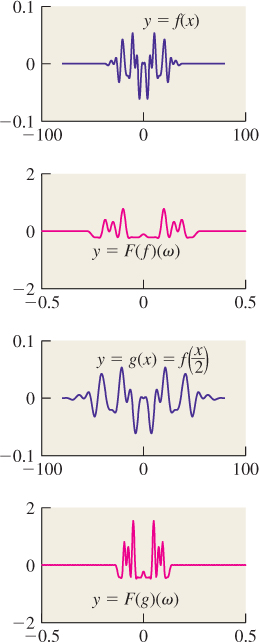
Figure 18.50: When we stretch the graph of f on the x-axis, the graph of ![]() (f) (in magenta) compresses on the ω-axis and stretches on the y-axis.
(f) (in magenta) compresses on the ω-axis and stretches on the y-axis.
Like most linear transformations, the Fourier transform is continuous; this means that if a sequence of functions fn approaches a function g, then ![]() (fn) approaches
(fn) approaches ![]() (g), assuming that both the f’s and the g are all in L2.
(g), assuming that both the f’s and the g are all in L2.
The Fourier transform has two final properties that make it important to us. The first is that it’s length-preserving, that is,
for every f ![]() L2(R). The proof is a messy tracing through definitions, with some careful fiddling with limits in the middle.
L2(R). The proof is a messy tracing through definitions, with some careful fiddling with limits in the middle.
The second property, whose proof is similar but messier, is the convolution-multiplication theorem. It states that
for any f, g ![]() L2(R). The same formulas apply when the Fourier transform is replaced by the inverse Fourier transform. The second formula also applies to functions defined on the interval H, or periodic functions of period one, although the convolution on the right is a convolution of sequences instead of a convolution of functions on the real line.
L2(R). The same formulas apply when the Fourier transform is replaced by the inverse Fourier transform. The second formula also applies to functions defined on the interval H, or periodic functions of period one, although the convolution on the right is a convolution of sequences instead of a convolution of functions on the real line.
![]() The convolution-multiplication function explains why it’s generally difficult to deconvolve. Suppose that
The convolution-multiplication function explains why it’s generally difficult to deconvolve. Suppose that ![]() is everywhere nonzero. Then convolving with g turns into multiplication by
is everywhere nonzero. Then convolving with g turns into multiplication by ![]() in the frequency domain. If we let h = f
in the frequency domain. If we let h = f ![]() g, then
g, then ![]() =
= ![]()
![]() . Now suppose we let u = 1/
. Now suppose we let u = 1/![]() . Multiplying
. Multiplying ![]() by u gives
by u gives ![]() . If U is the inverse Fourier transform of u, then convolving h with U will recover f, by the convolution-multiplication theorem. There is one problem in this formulation, however: If
. If U is the inverse Fourier transform of u, then convolving h with U will recover f, by the convolution-multiplication theorem. There is one problem in this formulation, however: If ![]() is an L2 function, then u = 1/
is an L2 function, then u = 1/![]() is generally not an L2 function. But it may be well approximated by an L2 function, so an approximate deconvolution is possible. On the other hand, suppose that
is generally not an L2 function. But it may be well approximated by an L2 function, so an approximate deconvolution is possible. On the other hand, suppose that ![]() (ω0) = 0 for some ω0. Then it’s impossible to even define u, let alone take its inverse transform. Roughly speaking, filtering by g removes all frequency-ω0 content from f, and there’s nothing we can do to recover that content later from the filtered result h.
(ω0) = 0 for some ω0. Then it’s impossible to even define u, let alone take its inverse transform. Roughly speaking, filtering by g removes all frequency-ω0 content from f, and there’s nothing we can do to recover that content later from the filtered result h.
18.18. Applications
We’ve defined two kinds of Fourier transform, and have observed that they are linear, continuous, and length-preserving, and satisfy the multiplication-convolution theorem. We can think of the Fourier transform as taking a “value representation” of a function f (i.e., the usual representation, where f (x) is the value of f at the location x) into a “frequency representation,” where ![]() (f)(ω) tells us “how much f looks like a sinusoid of frequency ω.”
(f)(ω) tells us “how much f looks like a sinusoid of frequency ω.”
We’ll now look at two applications of these ideas: band limiting and sampling.
18.18.1. Band Limiting
We’ve said that a function g is band-limited at ω0 if ![]() (g)(ω) = 0 for ω > ω0, that is “if g contains only frequencies up to ω0.” This is illustrated schematically in Figures 18.51 and 18.52. For the remainder of this section, we’ll fix ω0 so that “band-limited” means “band-limited at ω0.”
(g)(ω) = 0 for ω > ω0, that is “if g contains only frequencies up to ω0.” This is illustrated schematically in Figures 18.51 and 18.52. For the remainder of this section, we’ll fix ω0 so that “band-limited” means “band-limited at ω0.”

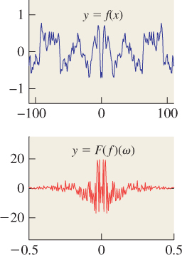
Now we’ll consider a similar computation on the interval H. Before we do so, we need one further fact: Just as the Fourier transform of a box was a sinc function, the inverse transform of a box is also a sinc function, as you can check by writing out the integrals.
Now suppose that f is a function in L2(H). What band-limited function g is closest to f? We’ll answer this using the Fourier transform. Figure 18.53 shows the idea. In the top row we see f and its transform. It’s mostly made up of frequencies less than 30, so we’ve truncated the transform to show the interesting parts. If we remove all the high frequencies (we’ve kept frequencies 17 and lower in this example), we get the function in the lower right. Removing all those frequencies amounts to multiplying by a box of width 34 (ranging from ω = –17 to ω = +17), that is, the function
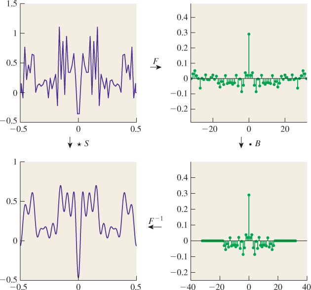
Figure 18.53: To get from ![]() to
to ![]() , we multiply by a box B(ω) = b(
, we multiply by a box B(ω) = b(![]() ); in other words, we remove all high frequencies. To get from f to g, we convolve with the inverse transform of B, namely a sinc of width 1/34, that is, x
); in other words, we remove all high frequencies. To get from f to g, we convolve with the inverse transform of B, namely a sinc of width 1/34, that is, x ![]() 34 sinc(34 x).
34 sinc(34 x).
Since multiplication by a box in the frequency domain is the same as convolution by a sinc in the value domain, the inverse transform of the lower-right signal, shown at the lower left, can also be obtained by convolving the original signal with an appropriately scaled sinc, namely
Notice that the result is a far smoother signal, g.
The signal g appears quite similar to the original signal f. It is in fact the band-limited signal that’s closest to f. That’s easy to see by looking on the right-hand side of the figure. The Fourier transform is distance preserving, that is, the distance between f and g is the distance between ![]() =
= ![]() (f) and
(f) and ![]() =
= ![]() (g). So to find the band-limited function closest to f, we need only look for the transform that is closest to
(g). So to find the band-limited function closest to f, we need only look for the transform that is closest to ![]() , but is zero outside the band limit. The only freedom we have in picking
, but is zero outside the band limit. The only freedom we have in picking ![]() is to adjust it between frequencies –17 and +17; by making it match
is to adjust it between frequencies –17 and +17; by making it match ![]() there, we make the difference of
there, we make the difference of ![]() and
and ![]() as small as possible.
as small as possible.
There’s nothing special about the number 17 in this example. We can “band-limit” the function f ![]() L2(H) at any frequency ω0.
L2(H) at any frequency ω0.
We can summarize the preceding two pages: If f is a function in L2(H), then to band-limit f at frequency ω0 we must convolve it with the function x ![]() S(x) = 2ω0 sinc(2ω0x), or, correspondingly, multiply its Fourier transform by
S(x) = 2ω0 sinc(2ω0x), or, correspondingly, multiply its Fourier transform by ![]() . The result is the band-limited function g that’s closest to f.
. The result is the band-limited function g that’s closest to f.
If you’re thinking to yourself, “Gosh, computing the convolution involves an integral, and doing that at every single point sounds really expensive,” you’re right. Fortunately, we’ll never need to actually do this in practice.
18.18.2. Explaining Replication in the Spectrum
As a second application, let’s revisit what we saw in Figure 18.45: When we multiplied the Taj Mahal data by a “sampling” function, the Fourier transform began to look periodic, as if it were made of multiple copies of the original transform, overlaid and summed up.
Figure 18.54 shows the situation, which we now explain. Let’s say that the original Taj Mahal data is described by a function x ![]() f(x). The “sampled” version, which we’ll call h, was generated by multiplying f by a function g that approximated a comb function, that is, that consisted of a bunch of narrow peaks of area 1, with spacing about 1/200, to produce a signal h = fg. This means that
f(x). The “sampled” version, which we’ll call h, was generated by multiplying f by a function g that approximated a comb function, that is, that consisted of a bunch of narrow peaks of area 1, with spacing about 1/200, to produce a signal h = fg. This means that ![]() =
= ![]()
![]()
![]() . But since g is an approximation of the comb function, its Fourier transform is an approximation of the transformed comb function, which is just another comb function. Since the spacing for g is about 1/200, the spacing for
. But since g is an approximation of the comb function, its Fourier transform is an approximation of the transformed comb function, which is just another comb function. Since the spacing for g is about 1/200, the spacing for ![]() is about 200. So
is about 200. So ![]() is just
is just ![]() convolved with a comblike function with spacing of 200. That convolution consists of multiple copies of
convolved with a comblike function with spacing of 200. That convolution consists of multiple copies of ![]() , one at each comb tooth, summed up. This explains the approximate periodicity of the Fourier transform
, one at each comb tooth, summed up. This explains the approximate periodicity of the Fourier transform ![]() .
.
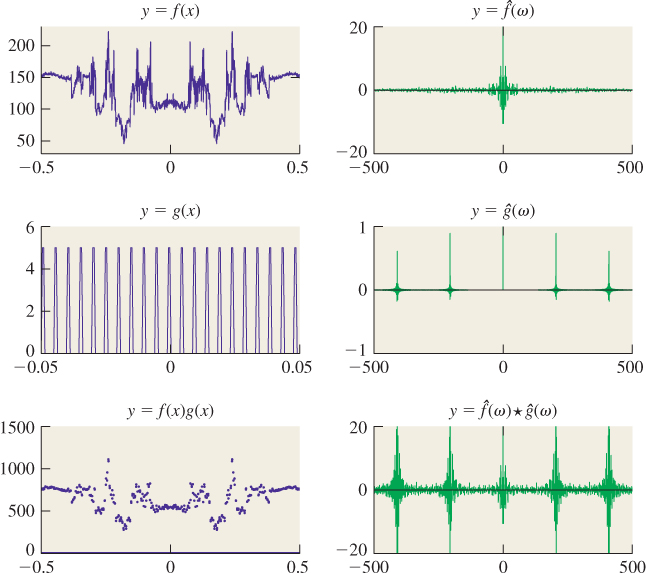
Figure 18.54: The Taj Mahal data (top left) is multiplied by a narrow comblike function (left middle—note the different scale on the x-axis!), with closely spaced peaks, to produce the “sampled” version at the bottom left. The Fourier transform of the original signal (top right) is convolved with the transform of the comblike signal (middle right, comblike with widely spaced peaks) to produce the transform of the sampled signal (bottom right), showing overlapping replicates of the transform of the original signal.
18.19. Reconstruction and Band Limiting
We now further examine the relationship between a function, f ![]() L2(R), and its samples at integer points, which define a function
L2(R), and its samples at integer points, which define a function ![]()
![]()
![]() 2(Z). We need a new definition: f is strictly band-limited at ω if
2(Z). We need a new definition: f is strictly band-limited at ω if ![]() (ω) = 0 for ω ≥ ω0. Note the shift from “>” to “≥.” The main result of this section is as follows.
(ω) = 0 for ω ≥ ω0. Note the shift from “>” to “≥.” The main result of this section is as follows.
• If ![]() (f)(ω) = 0 for |ω| ≥ 1/2, then f can be recovered from
(f)(ω) = 0 for |ω| ≥ 1/2, then f can be recovered from ![]() , that is, the map f
, that is, the map f ![]()
![]() is invertible once the domain is restricted to the functions strictly band-limited at 1/2.
is invertible once the domain is restricted to the functions strictly band-limited at 1/2.
• For any function g ![]()
![]() 2, there are multiple functions whose samples are given by g, so in general, it’s impossible to reconstruct an arbitrary L2 function from its samples.
2, there are multiple functions whose samples are given by g, so in general, it’s impossible to reconstruct an arbitrary L2 function from its samples.
The corresponding statements hold for a function f ![]() L2(H), sampled at a collection of n evenly spaced points in the interval; in that case, if the function is band-limited at any frequency below n/2, then it’s reconstructible from its samples. (Indeed, that’s the essence of the sampling theorem.)
L2(H), sampled at a collection of n evenly spaced points in the interval; in that case, if the function is band-limited at any frequency below n/2, then it’s reconstructible from its samples. (Indeed, that’s the essence of the sampling theorem.)
We’ll actually show exactly how to reconstruct a band-limited function from its samples, in that rather than just showing that the sampling process is invertible, we’ll explicitly describe an inverse. We’ll also describe some approximations to the inverse that are easily computable, that is, functions with the property that if f is band-limited, then sampling f, followed by the approximate-reconstruction operation, will yield a function very close to f.
We’ll start with the easy part: showing there are multiple functions with the same samples. Recall that for a continuous function, “sampling at x” simply means “evaluating the function at x.” So to show that there are two different functions with the same samples at integer points, consider f1(x) = 0 and f2(x) = sin(πx). At every integer point, these two have exactly the same value (namely 0). Thus, if you’re given the samples of one of the two functions, you cannot possibly tell which one it was. Of course, f2 isn’t in L2(R), because it doesn’t approach zero as x ![]() ±∞, but this quibble is easily resolved:
±∞, but this quibble is easily resolved:
Show that if f is any function in L2, then x ![]() f (x) f2(x) is a function whose samples match those of f1, so the sampling operation is a many-to-one map from L2(R)
f (x) f2(x) is a function whose samples match those of f1, so the sampling operation is a many-to-one map from L2(R) ![]()
![]() 2(Z).
2(Z).
Note, however, that the function f2 has frequency ![]() , so it’s just above the Nyquist limit: We expect it to produce aliasing.
, so it’s just above the Nyquist limit: We expect it to produce aliasing.
For the corresponding situation on the interval H = (–![]() ,
, ![]() ], a similar example suffices. If we consider the n equally spaced sample points xj = –
], a similar example suffices. If we consider the n equally spaced sample points xj = –![]() +
+ ![]() , j = 0, 1, . . ., n – 1, then the function g1(x) = 0 and the function g2(x) = sin(πn(x+
, j = 0, 1, . . ., n – 1, then the function g1(x) = 0 and the function g2(x) = sin(πn(x+![]() )) both take on the value 0 at every xj.
)) both take on the value 0 at every xj.
We say that the function g2 is an alias of the function g1, because from the point of view of their samples, they appear to be the same. If we had a way to construct a function on the whole interval from a set of samples, then the samples of g1 and g2, being identical, would produce identical results.
Now let’s turn to the more difficult part: showing that if a function is appropriately band-limited, it can be reconstructed from its samples.
As we saw earlier, if we have a function f ![]() L2(R) and multiply it by a “comblike” function in L2, the Fourier transform of the result starts to look periodic, consisting of multiple copies of the transform of f. As we take better and better approximations of the comb, the Fourier transform becomes closer and closer to the convolution of
L2(R) and multiply it by a “comblike” function in L2, the Fourier transform of the result starts to look periodic, consisting of multiple copies of the transform of f. As we take better and better approximations of the comb, the Fourier transform becomes closer and closer to the convolution of ![]() with a comb. The limit of the comb approximations doesn’t exist, of course, but the collection of samples of f does exist, and is a function
with a comb. The limit of the comb approximations doesn’t exist, of course, but the collection of samples of f does exist, and is a function ![]() in
in ![]() 2. In the frequency domain, the Fourier transforms of the convolutions of f with more and more comblike approximations of the comb get closer and closer to a periodic function. The limit is a periodic function, but that’s not in L2(R), because it doesn’t go to zero as ω
2. In the frequency domain, the Fourier transforms of the convolutions of f with more and more comblike approximations of the comb get closer and closer to a periodic function. The limit is a periodic function, but that’s not in L2(R), because it doesn’t go to zero as ω ![]() ±∞. On the other hand, it turns out that this periodic
±∞. On the other hand, it turns out that this periodic ![]() limit is the Fourier transform of
limit is the Fourier transform of ![]() . The proof of these claims is quite subtle; Dym and McKean [DM85] provide the necessary details for those who have studied real analysis.
. The proof of these claims is quite subtle; Dym and McKean [DM85] provide the necessary details for those who have studied real analysis.
To summarize the preceding paragraph briefly, if we take an L2(R) function f and sample it at integer points to get ![]()
![]()
![]() 2(Z), then
2(Z), then
where ψ is the comb function.
Suppose that f is strictly band-limited, that is, ![]() (f)(ω) = 0 for |ω| ≥
(f)(ω) = 0 for |ω| ≥ ![]() . Then
. Then ![]() (
(![]() ) consists of disjoint replicates of
) consists of disjoint replicates of ![]() (f). To recover the Fourier transform of f from this, we need only multiply it by a box of width 1, which is the function b. Multiplication by b in the frequency domain corresponds to convolution with
(f). To recover the Fourier transform of f from this, we need only multiply it by a box of width 1, which is the function b. Multiplication by b in the frequency domain corresponds to convolution with ![]() –1(b) in the value domain. The inverse Fourier transform of b is the function x
–1(b) in the value domain. The inverse Fourier transform of b is the function x ![]() sinc(x). We conclude that to reconstruct a band-limited function from its samples, it suffices to convolve the samples with sinc.
sinc(x). We conclude that to reconstruct a band-limited function from its samples, it suffices to convolve the samples with sinc.
This is a pretty big result. It says, for instance, that if you have an image created by sampling a band-limited function f, you can recover f from the image by convolving with a sinc. In one dimension, that means that if the samples are called fj, you can compute
If x happens to be an integer—say, x = 3—then this sum becomes
The arguments to sinc in this sum are all integers, and sinc is 0 at every integer point, except that sinc(0) = 1. So the sum simplifies to say
That’s good: It says that to reconstruct the value of f at an integer point, you just need to look at the sample there. What if x is not an integer? Then the sinc is nonzero at every argument, and the value of f at x involves a sum of infinitely many terms. This is clearly not practical to implement.
We’ll soon discuss other approaches to reconstruction, but the central idea—that we can reconstruct a function from its samples by convolving with sinc—remains important. We’ll use it repeatedly in the next chapter when we discuss shrinking and enlarging images. Typically we’ll apply this theoretical result multiple times to determine what computation we should be doing, and then, with the ideal computation at hand, we’ll determine a good approximation.
We’ve now seen two applications of convolving with sinc. The first is that for any function f ![]() L2(R), f
L2(R), f ![]() sinc is the band-limited function closest to f. As you’ll recall, that’s because in the frequency domain, convolution with sinc becomes “multiplication by a box,” which removes all high frequencies from f, while leaving the low frequencies untouched. That’s the Fourier transform of the band-limited function closest to f, hence its inverse transform is the band-limited function in the value domain closest to f. The second application is in reconstruction: To reconstruct a band-limited function from its samples, we convolve the samples with a sinc.
sinc is the band-limited function closest to f. As you’ll recall, that’s because in the frequency domain, convolution with sinc becomes “multiplication by a box,” which removes all high frequencies from f, while leaving the low frequencies untouched. That’s the Fourier transform of the band-limited function closest to f, hence its inverse transform is the band-limited function in the value domain closest to f. The second application is in reconstruction: To reconstruct a band-limited function from its samples, we convolve the samples with a sinc.
When we take a function and sample it as shown in Figure 18.55, it’s natural, when viewing the samples, to mentally “connect the dots,” as in Figure 18.56. We’ll now study how this compares with reconstruction with sinc.
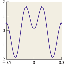
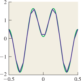
The first step is to recognize that “connecting the dots” gives the same results as convolving with the “tent function” b1 of Figure 18.57. When we remember that b1 = b ![]() b, we can see that connect-the-dots reconstruction is really just “convolve with b twice.”
b, we can see that connect-the-dots reconstruction is really just “convolve with b twice.”
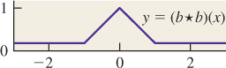
How does that look in the frequency domain? Ideally, we want to multiply by the unit-width box b in the frequency domain to get rid of all too-high frequencies. What we’re doing instead is multiplying by ![]() (b) = sinc twice—in other words, we’re multiplying by sinc2. How does this compare to multiplying by a box? Figure 18.58 shows the two functions, and you can see that they’re somewhat similar. Because sinc2 is nonzero for frequencies greater than
(b) = sinc twice—in other words, we’re multiplying by sinc2. How does this compare to multiplying by a box? Figure 18.58 shows the two functions, and you can see that they’re somewhat similar. Because sinc2 is nonzero for frequencies greater than ![]() , it does allow some high-frequency components of f to masquerade as low-frequency components. But the peak of ω
, it does allow some high-frequency components of f to masquerade as low-frequency components. But the peak of ω ![]() sinc2(ω) outside ω ≤
sinc2(ω) outside ω ≤ ![]() occurs at about ω ≈ 1.43, where the value is about 0.047, that is, at most 5% of any too-high frequency manages to survive as an alias. Thus, sinc2 does a decent job of band limiting. But what about its effects on frequencies that are low enough, that is, those that should be unattenuated? As we approach ω =
occurs at about ω ≈ 1.43, where the value is about 0.047, that is, at most 5% of any too-high frequency manages to survive as an alias. Thus, sinc2 does a decent job of band limiting. But what about its effects on frequencies that are low enough, that is, those that should be unattenuated? As we approach ω = ![]() from below, sinc2 falls off fairly rapidly. In fact, sinc2(
from below, sinc2 falls off fairly rapidly. In fact, sinc2(![]() ) ≈ 0.23, so signals near the Nyquist limit are attenuated to about one-quarter of the ideal. But by half the Nyquist limit, the attenuation is only about 20%. We should expect connect-the-dots reconstruction to work well in this region, but badly at or a little above the Nyquist limit.
) ≈ 0.23, so signals near the Nyquist limit are attenuated to about one-quarter of the ideal. But by half the Nyquist limit, the attenuation is only about 20%. We should expect connect-the-dots reconstruction to work well in this region, but badly at or a little above the Nyquist limit.
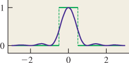
Clearly if we were to convolve the tent function b1 with the box b once more to get a new function b2, its Fourier transform would be sinc3, and it would better approximate the ideal box. On the other hand, convolving with the function b2 would involve blending together not just two samples, but three.
In the value domain, we can regard the tent function as an approximation of the sinc. The tent looks somewhat like the central hump of the sinc, and hence their transforms are somewhat similar. Pursuing this idea, we could produce a piecewise quadratic or piecewise cubic function that better fit the first few lobes of the sinc, and whose Fourier transform would therefore be more like a box. Such an approximation is what’s used by image-manipulation programs like Adobe Photoshop when the user selects “bicubic” interpolation.
When we display an image on an LCD monitor, we effectively take the sample values and use them to control the intensity of a square display pixel. The analog in one dimension is that we take each sample and expand it into a unit-width constant function, that is, we convolve the sampled signal with the box function b. In the frequency domain, that means we’re multiplying by sinc once, which is much less effective at band-limiting the signal than multiplying by sinc2. The result is more substantial aliasing than in the case of the tent reconstruction.
18.20. Aliasing Revisited
In Section 18.2, we discussed line rendering for a grayscale LCD monitor using rounding, unweighted area sampling, and weighted area sampling. We’ll now reexamine each approach using the value-frequency duality.
First, following the book’s first principle—Know Your Problem—let’s state the problem clearly. Given a line y = mx + b with slope 0 < m < 1, there’s a function f that’s 1 for any point (x, y) whose distance to the line is less than ![]() , and 0 otherwise. This function can be described as the “Am I in a unit-width stripe defined by y = mx + b” function. This function has sharp transitions from black to white (or 0 to 1), so its (two-dimensional) Fourier transform contains arbitrarily high frequencies. In fact, any horizontal slice of this function (i.e., x
, and 0 otherwise. This function can be described as the “Am I in a unit-width stripe defined by y = mx + b” function. This function has sharp transitions from black to white (or 0 to 1), so its (two-dimensional) Fourier transform contains arbitrarily high frequencies. In fact, any horizontal slice of this function (i.e., x ![]() f (x, y0)) looks like a bump of some width, and hence its 1D Fourier transform looks like a sinc, which is nonzero for arbitrarily high frequencies. The function f is not in L2(R2), but outside the image we’re going to render—say, a 100×100 image—we can define f to be 0, and then it will be in L2. Our goal is to have the pattern of light emitted by the display be as near to a band-limited approximation of f (or a multiple of it, to deal with units) as possible.
f (x, y0)) looks like a bump of some width, and hence its 1D Fourier transform looks like a sinc, which is nonzero for arbitrarily high frequencies. The function f is not in L2(R2), but outside the image we’re going to render—say, a 100×100 image—we can define f to be 0, and then it will be in L2. Our goal is to have the pattern of light emitted by the display be as near to a band-limited approximation of f (or a multiple of it, to deal with units) as possible.
The “rounding” approach turns out to be equivalent to sampling a slightly fatter version of the function f : The pixel (x, y) is “illuminated” if its vertical distance to y = mx + b is no more than ![]() . The samples of this function constitute an
. The samples of this function constitute an ![]() 2 function on the integer grid. Its spectrum is the result of convolving the spectrum of f with a two-dimensional comb, resulting in many high-frequency components aliasing as low-frequency ones. Displaying these samples on the LCD monitor amounts to convolving the image with a 2D box function, that is, multiplying by a (2D) sinc in the frequency domain. So the rounding approach, in the frequency domain, looks like convolution with a comb, followed by multiplication by a sinc. The end result is nowhere near a band-limited approximation of the function f, and the result, as we saw, looks bad.
2 function on the integer grid. Its spectrum is the result of convolving the spectrum of f with a two-dimensional comb, resulting in many high-frequency components aliasing as low-frequency ones. Displaying these samples on the LCD monitor amounts to convolving the image with a 2D box function, that is, multiplying by a (2D) sinc in the frequency domain. So the rounding approach, in the frequency domain, looks like convolution with a comb, followed by multiplication by a sinc. The end result is nowhere near a band-limited approximation of the function f, and the result, as we saw, looks bad.
In the next approach to line rendering, there were three steps.
1. Convolve with a 2D box to compute area overlaps.
2. Sample at integer points.
3. Convolve with a 2D box to display.
In frequency space, we multiply ![]() (f) by a sinc, convolve with a 2D comb, and then multiply by sinc again. As we already saw, multiplying f by sinc weakly band-limits it—too-high frequencies are attenuated, although not perfectly. Convolution with the comb introduces the high-frequency parts that passed the weak band limiting as low-frequency aliases. And multiplying by sinc again weakly band-limits the results. The effect of the extra sinc in the first step is noticeable, and the grayscale line rendering is far nicer.
(f) by a sinc, convolve with a 2D comb, and then multiply by sinc again. As we already saw, multiplying f by sinc weakly band-limits it—too-high frequencies are attenuated, although not perfectly. Convolution with the comb introduces the high-frequency parts that passed the weak band limiting as low-frequency aliases. And multiplying by sinc again weakly band-limits the results. The effect of the extra sinc in the first step is noticeable, and the grayscale line rendering is far nicer.
In weighted area sampling, the first step is replaced by convolution with a 2D tent rather than a 2D box; in the frequency domain, we’re multiplying by sinc2, which is a far more effective band limiter. The final results are correspondingly better.
In the last two cases, we’ve only approximately band-limited during the sampling process; in the first one, we never band-limited at all. And in all cases, the display process produces an image that contains a great many high frequencies at the edges between display pixels. But we have, at least in the last two cases, got an approximation of the ideal solution.
Or have we? We’ve actually failed in three ways. First, the notion of “nearness” used in this chapter is the L2 distance, and we’ve already mentioned that this doesn’t actually correspond very closely to a perceptual notion of similarity of images, so it’s possible that we’ve optimized for the wrong thing. Second, we’ve been concerned about high frequencies, but in practice, once the pixels are small enough that the high-frequency components of the pattern of emitted light are so high-frequency that we cannot detect them with our eyes, these high frequencies don’t matter. Of course, a high frequency that aliases to a low frequency that we can detect does matter. But if some line-rendering approach leaves in a few components that are just above the Nyquist limit, their aliases will be just below the Nyquist limit, which may be well above the range of frequencies our eyes can detect, and therefore may not matter at all.
The third failure is of a larger kind: We’ve taken the view that we must first band-limit, then sample, then reconstruct, and we’ve looked at each step separately, and accepted approximations in each one. To some degree, we’ve approximated the steps of the solution rather than the solution itself violating the Approximate the Solution Principle. Here’s an alternative problem to consider: Among all possible patterns of light that the display can produce, which one is L2 closest to the function f? If we know that we’re going to be displaying the result on a square-pixel LCD screen, isn’t this a reasonable question to be asking? It turns out that the solution to this “nearest displayable image” problem is produced by unweighted area sampling. But actually using unweighted area sampling generates some interesting artifacts of its own: Vertical and horizontal lines look sharper, indeed are sharper, than diagonal ones, and lines in horizontal motion appear to speed up and slow down as we saw in the case of the moving triangle at the start of the chapter. Does this matter? That depends on our eyes’ ability to detect variations in speed of motion for various speeds. You might want to write a program to experiment with this and draw your own conclusions. The real lesson of this example is that it’s worth thinking about sampling and reconstruction together rather than as separate processes.
18.21. Discussion and Further Reading
If we want an image (i.e., a rectangular array of samples from some function f) to be faithfully reconstructible (i.e., we want to be able to recover f from the samples), then the process that generated the image must be lossless (i.e., an invertible map of vector spaces). In general, this requires that we restrict the original function to some subset of L2, and the usual choice is “the band-limited functions.”
Unfortunately, in practice we’re often confronted with functions we’d like to sample but which are not band-limited. The solution is to find a way to convert such a function f into a nearby function f0 that is band-limited. The ideal way to do so is to convolve f with a sinc, but that’s impractical in general. Convolving with other, simpler, filters like the box can give a decent approximation.
In practice, this means that if you want to write a ray tracer, you shouldn’t just sample one ray at the center of each pixel. Instead, you should shoot many rays per pixel and average them. This is a low-budget approximation of box-filtering the “incoming light” function. Alternatively, you could compute a weighted sum of the ray values, approximating the convolution of the incoming light with some filter like the sinc or the tent, or any other filter you like.
Although the sinc filter is the ideal “low-pass” filter, it has some problems in practice. If you have a wide box function, for instance, and you filter it with sinc, the result contains ringing—little wiggles on either side of the discontinuity. That’s not “wrong” in any sense, but it presents a problem for display: Because some of the resultant values are negative, you want to make those parts of your display “even blacker than black,” which is impractical. This is yet another reason to favor a tent filter, or some other everywhere-positive approximation of a sinc.
The idea that “details below the scale of our eyes’ ability to detect them don’t matter” can be used in an interesting way: The three colored strips in a typical LCD display pixel can be individually adjusted in ways that give finer control than adjusting all three together, even for a grayscale image. For instance, the antialiased letter “A” shown in Figure 18.14 was originally rendered this way; Figure 18.59 shows how it looked. This technology, used in font rendering, is called TrueType [BBD+99]. Ideas like this can surely be used in other ways in graphics as well.

The Nyquist limit, from the discussion in this chapter, appears to be absolute: You can’t sample signals with frequencies above the Nyquist limit and hope to reconstruct them. But that’s not completely true. Suppose that the Nyquist frequency for some sampling rate is ω0. Then a signal whose Fourier transform is nonzero strictly between –ω0 and ω0 can be perfectly reconstructed from its samples. But it’s also the case that a signal whose Fourier transform is nonzero strictly between 5ω0 and 7ω0 can be perfectly reconstructed from its samples, provided we know at the time of reconstruction these limits on the transform. Indeed, if we know the samples of a function f and we know an interval I of length 2ω0 with the property that f’s transform is nonzero only strictly within I, then we can reconstruct f. Similarly, if we know that the transform of f is sparse—that is, nonzero at relatively few points—we can use this sparsity to reconstruct f even if its transform is not constrained to an interval of length ω0. This is part of the subject of the relatively new field of compressive sensing [TD06].
We started this chapter by saying that every L2 function on an interval can be (nearly) written as a sum of sines and cosines. You might reasonably ask, “Why sines and cosines? Why not boxes of varying width, or tentlike functions, or some other collection of functions?” The first answer, which we’ll return to in a moment, is that you can write an L2 function as a sum of things other than sines and cosines, and it’s often worthwhile to do so. But the Fourier decomposition has proven widely useful in engineering, mathematics, and physics. Why? One answer is based on the principle that if you have a linear transformation from a space to itself, it’s often easiest to understand that transformation when you change to a basis made up of eigenvectors, for then the transformation is just a nonuniform scaling transformation. Many of the laws of physics appear as second-order linear differential equations, like F = ma, in which the unknown position x is described by saying that its second derivative, a, must satisfy F = ma, where the mass m and the force F are typically known, and x is required to satisfy some boundary conditions as well. In the event that F and m are constant over time, this is a second-order equation with constant coefficients. The solutions to such equations can be generally written as sums of exponentials, where the exponent may be real or complex. The complex case leads to sines and cosines. Thus, expressing things as a sum of sines and cosines arises naturally because of the world’s defining equations being second-order linear equations. In fact, Fourier introduced the transform in the process of describing how to solve the heat equation, which describes how the heat in a solid evolves over time in response to initial and boundary conditions.
Oppenheim and Schaefer [OS09] make a similar case for discrete signals, saying that every linear shift-invariant system has, as its fundamental solutions, combinations of sines and cosines. Shift-invariant in this context means that if you regard the system as one that takes an input signal that’s a function of t and produces an output signal that’s another function of t, then delaying the input (i.e., shifting from t ![]() s(t) to t
s(t) to t ![]() s(t – h)) produces the exact same output, but shifted by the same amount. In physical terms, it says that the system will behave the same way tomorrow that it does today.
s(t – h)) produces the exact same output, but shifted by the same amount. In physical terms, it says that the system will behave the same way tomorrow that it does today.
We return now to the first answer—that you can write functions as sums of things other than sines and cosines. Two of the key features of the Fourier decomposition are localization in frequency and orthogonality. The first means that we can look at the Fourier transform of a signal and to the degree that the signal is mostly made up of one frequency, the Fourier transform will be small except at that frequency. The second means that the inner product of exp(inπx) and exp(ikπx) is 0 unless k = n; this means that it’s easy to write a function f in the Fourier basis by just computing the inner product of f with exp(inπx) for each n, and using the resultant numbers as coefficients in the linear combination.
In his 1909 dissertation under Hilbert, Haar showed that every L2 function on [0, 1] could be well approximated by a sum of functions that were constant on intervals of size 2–k (for k = 0, 1, 2, ...) and localized in space, that is, each function is nonzero only on two such intervals. These functions (and corresponding ones for larger k) are called the Haar wavelets. Figure 18.60 shows a few of the functions.
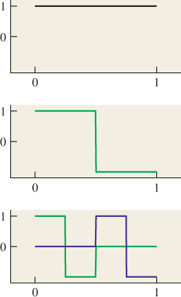
Figure 18.61 shows a function f on the unit interval, while Figure 18.62 shows an approximation of it that’s constant on intervals of length ![]() . Figure 18.63 shows how that approximation can be written as a linear combination of the Haar wavelets: The next-to-bottom row is the weighted sum of the k = 3 wavelets, each portion drawn in a different color; the next up is the sum of the k = 2 wavelets, etc. The top row is a constant function whose value is the average value of f on the interval. The height of the vertical red bar in the bottom row is the sum of the heights of the red bars in all rows above it.
. Figure 18.63 shows how that approximation can be written as a linear combination of the Haar wavelets: The next-to-bottom row is the weighted sum of the k = 3 wavelets, each portion drawn in a different color; the next up is the sum of the k = 2 wavelets, etc. The top row is a constant function whose value is the average value of f on the interval. The height of the vertical red bar in the bottom row is the sum of the heights of the red bars in all rows above it.
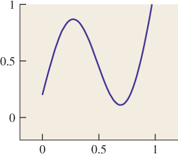
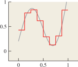
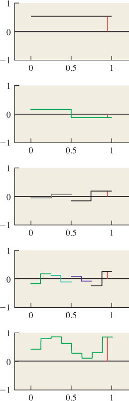
Figure 18.63: The approximation written as a sum of spatially localized functions of various scales.
If we take a limit and approximate the signal by such functions at finer and finer scales, the coefficients of the resultant (infinite) linear combination is called the Haar wavelet transform of the original function.
While Haar wavelets are conceptually very simple, and share some properties of the Fourier basis, they lack some others. For instance, they are not infinitely differentiable; indeed, they’re not even once-differentiable. In the mid-1990s, Haar wavelets, and several other more complex forms of wavelets, with varying degrees of smoothness, were widely adopted in computer graphics, with applications all the way from line drawing [FS94] to rendering [GSCH93]. For those who wish to learn more, we highly recommend Wavelets for Computer Graphics: A Primer, by Stollnitz et al. [SDS95], as a gentle introduction to the subject, motivated by examples from graphics.
By the way, there’s an analog to the Shannon theorem for Haar wavelets (or generally for any other basis in which you choose to write a function): If you have enough samples of a function that’s known to be a combination of a fixed number of certain basis functions, you can reconstruct the function. For some classes the locations of the samples may be restricted in various ways (e.g., for Haar wavelets, they should not be of the form p/2q, where p and q are integers), but the general idea still works.
The Fourier basis is a great way to represent one- and two-dimensional signals, but in graphics we also tend to encounter functions on the sphere, or on S2 × S2, like the BSDF. There’s an analogous basis for S2 called spherical harmonics, which we touch on briefly in Chapter 31. A nice introduction to these is provided by Sloan [Slo08].
18.22. Exercises
Exercise 18.1: (a) We defined the length || f|| for a function in L2. How do you know that the length of any function f ![]() L2 is finite?
L2 is finite?
(b) Show that || f + g||2 – || f||2 – || g||2 = 2 ![]() f, g
f, g![]() for any f, g
for any f, g ![]() L2, and conclude that the inner product of f and g is therefore always finite as well.
L2, and conclude that the inner product of f and g is therefore always finite as well.
Exercise 18.2: (An exercise in definitions.) Define ga(t) = ![]() for |t| < a and 0 otherwise.
for |t| < a and 0 otherwise.
(a) Show that for any function f : R ![]() R, the value U(a) defined in Equation 18.26 is (f
R, the value U(a) defined in Equation 18.26 is (f ![]() ga)(t0).
ga)(t0).
(b) Show that the sample of f at t0 is lima![]() 0(f
0(f ![]() ga)(t0).
ga)(t0).