
Chapter 17. Image Representation and Manipulation
17.1. Introduction
Digital imagery appears in all forms of media today. Although most of these images are digital photos or other types of 2D pictures that have been loaded or scanned into a computer, an increasing number of them are generated in 3D using sophisticated modeling and rendering software. Accompanying this trend is a large number of image formats, most of which are interconvertible (albeit with some loss of fidelity). Images in each format have limitations, especially in their ability to represent wide ranges of intensity; as a result, new formats for high dynamic range (HDR) images have also evolved. Because most images come from digital cameras, it’s natural to think of each pixel as storing a red, a green, and a blue value (an RGB format), and then using the values to drive the red, green, and blue colors of a screen pixel when the image is displayed. But in practice, especially with digital images, each pixel is likely to contain considerably more information. The pixel may also contain a depth value representing distance from the virtual camera, an alpha value representing a kind of transparency, and even values like an identifying constant that tells what object is visible in this pixel.
In this chapter and the one that follows, we discuss how images are typically stored, and some techniques for manipulating them, including compositing. Then we examine the content of images more carefully, determining how much data an image can hold and what this says about the operations we can perform on it reliably. Finally, with this richer view of images, we discuss different forms of image transformation and take a look at their benefits and limitations.
17.2. What Is an Image?
We’ll start with a definition, which we’ll later refine somewhat: An image is a rectangular array of values, called pixel values, all of which have the same type. These pixel values may be real numbers representing levels of gray (a grayscale image), or they may be triples of numbers representing mixtures of red, green, and blue (an RGB image),1 or they may contain, at each pixel, other information in addition to color or grayscale data; a rich example is so-called z-data, indicating at each pixel the distance from the viewpoint from which the image was captured or produced.
1. The precise meanings of the red, green, and blue values may be quite vague; we’ll discuss this thoroughly later.
A rectangular array of numbers can be interpreted in many ways. For instance, it’s possible to display a z-data or depth image in grayscale, in which case the parts of the image that are near the viewer are displayed in lighter shades of gray than the parts that are far away. A priori, the numbers in the array have no particular significance. But for practical matters, when we take a digital photograph we’d like to know whether the pixels store red-green-blue triples or green-blue-red triples, since any confusion could cause very peculiar pictures to be displayed or printed. Thus, image data is typically stored in certain standard file formats, where the meaning of the data associated to each pixel is standardized. Some formats, notably TIFF (Tagged Image File Format), allow you to associate a description to each datum. For instance, the description of a TIFF file might be “Each pixel has five values associated to it: a red, green, and blue value represented by an integer ranging from 0 to 255, a z-value represented by an IEEE floating-point number, and an object identifier represented by a 16-bit unsigned integer.” With this in mind, we begin our discussion of images with the mundane and practical issue of how conventional file formats store and represent rectangular arrays of data.
How these rectangular arrays of values actually represent light intensities (or other physical phenomena) and how well they do so is also important. Following our discussion of image file formats, we move on to discuss the content of images.
17.2.1. The Information Stored in an Image
When we have a typical image file format, storing an n × k array of grayscale values or RGB triples, it’s natural to think about operations like adding together two images, pixel by pixel (or averaging them, pixel by pixel), to create effects like a cross-fade. To do such things requires a notion of addition of images and of multiplication by constants, which we take from the operations on each pixel (i.e., to add two images, we add corresponding pixel values). For grayscale images, what we have, in effect, is a correspondence between the set of n × k images and the elements of Rnk, given by enumerating the pixel values in some fixed order. Thus, the set of all images forms a subset of an nk-dimensional space.
Each element of the standard basis for Rnk consists of nk – 1 zeroes and a single one. What does the corresponding image look like? Can you see how you could represent every image as a sum of scalar multiples of such “basis images”?
Contrast this description of an n × k image with the scene you witness as you look through a window: At every point of the window, you perceive a color with some amount of lightness. That is to say, we could summarize your percept as a function from points of the window to real numbers representing lightness (measured in some way) at the points. The set of all real-valued functions on a rectangle constitutes an infinite-dimensional vector space. We choose, however, to represent such images with n × k representative numbers, that is, an element of a finite-dimensional vector space. There is necessarily some loss in the conversion from the former to the latter. The exact nature of this loss depends on how the finite image was created; we’ll see that the choices made during image formation (whether via a camera or via a software renderer) can have far-reaching impact.
17.3. Image File Formats
Images are stored in many formats; typically the storage format bears a close resemblance to the display format. That is, an n × k image may be stored as nk triples of RGB values, with each R value representing the red part of a pixel, stored in a sequence of some fixed number of bits, and similarly for G and B. But some formats have more complex representations. For example, we might, considering the red values only, reading across a row of an image, store the value of the first pixel, and the difference of the second from the first, and then the difference of the third from the second etc. Because these differences will tend to be smaller numbers, we might hope to store them with fewer bits. This would give a losslessly compressed image: one in which the data occupies less space, but from which the original RGB image can be reconstructed.
On the other hand, sometimes we can use lossy compression—a method of compressing an image so that some of the original data is lost, but not enough to matter for the intended use of the image. A simple lossy compression scheme would be to store only a checkerboard pattern of alternate pixels and then, at display time, interpolate missing pixel values from the known neighboring values. This generates a two-to-one savings in storage, but at a cost of substantial image-quality loss in many cases. More sophisticated compression schemes use the known statistics of natural images and known information about the human visual system (e.g., we’re sensitive to sharp edges, but less sensitive to slowly changing colors) to choose which data in the image to keep and omit. JPEG compression, for instance, divides the image into small blocks and compresses the data stored in each one; it’s easy to see the blocks if you zoom in on a displayed JPEG image.
Some formats also store metadata (information about when the image was produced, what device or program produced it, etc.) and, in some cases, information about the contents, which is typically described in terms of channels. The red values for all pixels constitute one channel, called a color channel; there are corresponding blue and green channels. The colors stored in one color channel may be represented by small integers with some number of bits, so we speak of an “8-bit red channel” or a “6-bit blue channel.” The image metadata gives information like the “bit depth” of each color channel. If the image also contains a depth value at each pixel, we speak of a “depth channel”; the metadata describes such noncolor channels as well.
17.3.1. Choosing an Image Format
Most digital cameras produce JPEG images; because of this, JPEG has become a de facto standard that is especially appropriate for natural images containing gray values or RGB values. On the other hand, the format is lossy, which makes it difficult to use when comparing images because it is impossible to know whether the images are really different from each other or whether minor underlying differences caused the JPEG compression algorithm to make different choices.
When image storage requirements were critical, and scanners and digital cameras were rare, a common format was GIF (Graphics Interchange Format), in which each pixel stored a number from 0 to 255, which was an index into a table of 256 colors. To create a GIF image, one had to decide which 256 colors to use, adjust each pixel to be one of these 256 colors, and then build the array of indices into the table. In images with just a few colors (some corporate logos, diagrams produced with simple drawing and painting tools, icons like arrows, etc.), the GIF format works beautifully; for natural images, it works rather poorly in general. Because one is only allowed 256 colors, the GIF representation is usually lossy.
As mentioned above, TIFF images store multiple channels, each with a description of its contents. For image editing and compositing tools, in which multiple layers of images are blended or laid atop one another, a TIFF image provides an ideal representation for intermediate (or final) results.
The PPM format, which you already encountered in Chapter 15, is very closely related to the organization of image data. In the text-based version of the format, one gives a “magic code” (namely P3), and then the width and height of the image (a pair of ASCII representations of positive integers w and h), the maximum color value (an integer no greater than 65,536), and then 3wh color values, representing the red, green, and blue components of the image pixels, in left-to-right, top-to-bottom order (so the first 3w numbers represent the colors in the top row of the image). Each color value must be no greater than the specified maximum color value, and is stored as an ASCII representation of the value. All values (including the width and height) are separated by whitespace. There’s also a binary version of the format (with magic code P5) in which the pixel data is stored in a binary representation, and there are also variants for storing grayscale images in text and binary formats.
One particular advantage of PPM is that the meaning of each pixel is, to a large degree, specified by the format. To quote the description:
[Pixel values] are proportional to the intensity of the CIE Rec. 709 red, green, and blue in the pixel, adjusted by the CIE Rec. 709 gamma transfer function. (That transfer function specifies a gamma number of 2.2 and has a linear section for small intensities). A value of Maxval for all three samples represents CIE D65 white and the most intense color in the color universe of which the image is part (the color universe is all the colors in all images to which this image might be compared) [Net09].
The CIE referred to in this description is the standards committee for color descriptions, discussed in detail in Chapter 28.
In recent years, the Portable Network Graphics or PNG format has become popular, in part because of patent issues with the GIF format. It is generally more compact than the naive PPM format, but it is equally easy to use.
For programs that manipulate images, the choice of image format is almost always irrelevant: You almost certainly want to represent an image as an array of double-precision floating-point numbers (or one such array per channel, or perhaps a single three-index array where the third index selects the channel). The reason to favor floating-point representations is that we often perform operations in which adjacent pixel values are averaged; averaging integer or fixed-point values, especially when it’s done repeatedly, may result in unacceptable accumulated roundoff errors.
There are two exceptions to the “use floating point” rule.
• If the data associated to each pixel is of a type for which averaging makes no sense (e.g., an object identifier telling which object is visible at that pixel—a so-called object ID channel), then it is better to store the value in a form for which arithmetic operations are undefined (such as enumerated types), as a preventive measure against silly programming errors.
• If the pixel data will be used in a search procedure, then a fixed-point representation may make more sense. If, for example, one is going to look through the image for all pixels whose neighborhoods “look like” the neighborhood of a given pixel, integer equality tests may make more sense than floating-point equality tests, which must almost always be implemented as “near-equality” tests (i.e., “Is the difference less than some small value ![]() ?”).
?”).
17.4. Image Compositing
Movie directors often want to film a scene in which actors are in some type of interesting situation (e.g., a remote country, a spaceship, an exploding building, etc.). In many cases, it’s not practical to have the actors actually be in these situations (e.g., for insurance reasons it’s impossible to arrange for top-paid actors to stand inside exploding buildings). Hollywood uses a technique called blue screening (see Figure 17.1) to address this. With this technique, the actors are recorded in a featureless room in which the back wall is of some known color (originally blue, now often green; we’ll use green in our description). From the resultant digital images, any pixel that’s all green is determined to be part of the background; pixels that have no green are “actor” pixels and those that are a mix of green and some other color are “part actor, part background” pixels. Then the interesting situation (e.g., the exploding building) is also recorded. Finally, the image of the actors is composited atop the images of the interesting situation: Every green pixel in the actor image is replaced by the color of the situation-image pixel; every nongreen pixel remains. And the partially green pixels are replaced by a combination of a color extracted from the actor image and the situation image (see Figure 17.2). The resultant composite appears to show the actor in front of the exploding building.
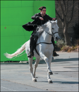
Figure 17.1: An actor, photographed in front of a green screen, is to be composited into a scene. (Jackson Lee/Splash News/Corbis)
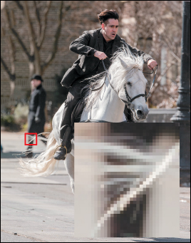
Figure 17.2: The actor, composited atop an outdoor scene. The detail shows how the horse’s tail obscures part of the background, while some background shows through. (Jackson Lee/Splash News/Corbis)
There are some limitations to this approach: The lighting on the actors does not come from the lighting in the situation (or it must be carefully choreographed to approximate it), and things like shadows present real difficulties. Furthermore, at the part actor, part background pixels, we have to estimate the color that’s to be associated to the actors, and the fraction of coverage. The result is a foreground image and a mask, whose pixel values indicate what fraction of the pixel is covered by foreground content: A pixel containing an actor has mask value 1; a pixel showing the background has mask value 0, and a pixel at the edge (e.g., in the actor’s hair) has some intermediate value.
In computer graphics, we often perform similar operations: We generate a rendering of some scene, and we want to place other objects (which we also render) into the scene after the fact. Porter and Duff [PD84] gave the first published description of the details of these operations, but they credit the ideas to prior work at the New York Institute of Technology. Fortunately, in computer graphics, as we render these foreground objects we can usually compute the mask value at the same time, rather than having to estimate it; after all, we know the exact geometry of our object and the virtual camera. The mask value in computer graphics is typically denoted by the letter α so that pixels are represented by a 4-tuple (R, G, B, α). Images with pixels of this form are referred to as RGBA images and as RGBα images.
Porter and Duff [PD84] describe a wide collection of image composition operations; we’ll follow their development after first concentrating on the single operation described above: If U and V are images, the image “U over V” corresponds to “actor over (i.e., in front of) situation.”
17.4.1. The Meaning of a Pixel During Image Compositing
The value α represents the opacity of a single pixel of the image. If we regard the image as being composed of tiny squares, then α = 0.75 for some square tells us that the square is three-quarters covered by some object (i.e., 3/4 opaque) but 1/4 uncovered (i.e., 1/4 transparent). Thus, if our rendering is of an object consisting of a single pure-red triangle whose interior covers three-quarters of some pixel, the α-value for that pixel would be 0.75, while the R value would indicate the intensity of the red light from the object, and G and B would be zero.
With a single number, α, we cannot indicate anything more than the opacity; we cannot, for instance, indicate whether it is the left or the right half of the pixel that is most covered, or whether it’s covered in a striped or polka-dot pattern. We therefore make the assumption that the coverage is uniformly distributed across the pixel: If you picked a point at random in the pixel, the probability that it is opaque rather than transparent is α. We make the further assumption that there is no correlation between these probabilities in the two images; that is, if αU = 0.5 and αV = 0.75, then the probability that a random point is opaque in both images is 0.5 · 0.75 = 0.375, and the probability that it is transparent in both is 0.125.
The red, green, and blue values represent the intensity of light that would arise from the pixel if it were fully opaque, that is, if α = 1.
17.4.2. Computing U over V
Because compositing is performed one pixel at a time, we can illustrate our computation with a single pixel. Figure 17.3 shows an example in which αU = 0.4 and αV = 0.3. The fraction of the image covered by both is 0.4 · 0.3 = 0.12, while the fraction covered by V but not U is 0.6 · 0.3 = 0.18.
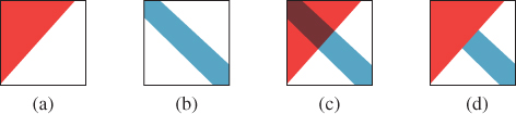
Figure 17.3: (a) A pixel from an image U, 40% covered. Properly speaking, the covered area should be shown scattered randomly about the pixel square. (b) A pixel from the image V, 30% covered. (c) The two pixels, drawn in a single square; the overlap area is 12% of the pixel. (d) The compositing result for U over V: All of the opaque part of U shows (covering 40% of the pixel), and the nonhidden opaque part of V shows (covering 18% of the pixel).
To compute U over V, we must assign both an α-value and a color to the resultant pixel. The coverage, α, will be 0.4 + 0.18, representing that all the opaque parts of U persist in the composite, as do the parts of V not obscured by U. In more generality, we have
What about the color of the resultant pixel (i.e., the intensity of red, green, and blue light)? Well, the light contributed by the U portion of the pixel (i.e., the fraction αU containing opaque bits from U) is αU · (RU, GU, BU), where the subscript indicates that these are the RGB values from the U pixel. The light contributed by the V part of the pixel is (1 – αU)αV · (RV, GV, BV). Thus, the total light is
while the total opacity is α = αU + (1 – αU)αV. If the pixel were totally opaque, the resultant light would be brighter by a factor of α; to avoid this brightness change, we must divide by α, so the RGB values for the pixel are
These compositing equations tell us how to associate an opacity or coverage value and a color to each pixel of the U over V composite.
17.4.3. Simplifying Compositing
Porter and Duff [PD84] observe that in these equations, the color of U always appears multiplied by αU, and similarly for V. Thus, if instead of storing the values (R, G, B, α) at each pixel, we stored (αR, αG, αB, α), the computations would simplify. Denoting these by (r, g, b, α) (so that r denotes Rα, for instance), the compositing equations become
α = 1 · αU + (1 – αU) · αV and
(r, g, b) = 1 · (rU, gU, bU) + (1 – αU) · (rV, gV, bV),
where the fraction has disappeared because the new (r, g, b) values must include the premultiplied α-value.
The form of these two equations is identical: The data for U are multiplied by 1, and the data for V are multiplied by (1 – αU). Calling these FU and FV, the “over” compositing rule becomes
17.4.4. Other Compositing Operations
Porter and Duff define other compositing operations as well; almost all have the same form as Equation 17.4, with the values FU and FV varying. One can think of each point of the pixel as being in the opaque part of neither U nor V, the opaque part of just U, of just V, or of both. For each, we can think of taking the color from U, from V, or from neither, but to use the color of V on a point where only U is opaque seems nonsensical, and similarly for the points that are transparent in both. Writing a quadruple to describe the chosen color, we have choices like (0, U, V, U) representing U over V and (0, U, V, 0) representing U xor V (i.e., show the part of the image that’s in either U or V but not both). Figure 17.4, following Porter and Duff, lists the possible operations, the associated quadruples, and the multipliers FA and FB associated to each. The table in the figure omits symmetric operations (i.e., we show U over V, but not V over U).
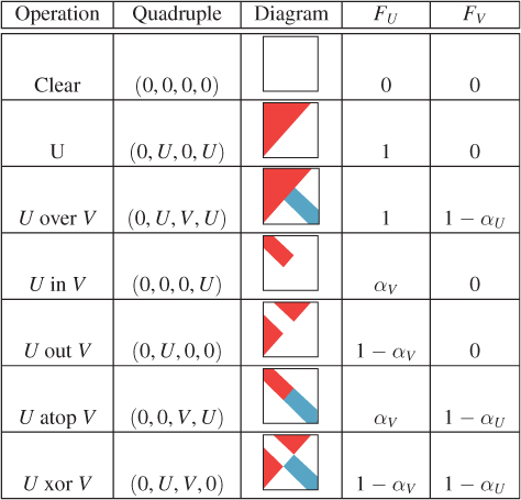
Figure 17.4: Compositing operations, and the multipliers for each, to be used with colors premultiplied by α (following Porter and Duff).
Finally, there are other compositing operations that do not follow the blending-by-Fs rule. One of these is the darken operation, which makes the opaque part of an image darker without changing the coverage:
Closely related is the dissolve operation, in which the pixel retains its color, but the coverage is gradually reduced:
Explain why, in the dissolve operation, we had to multiply the “rgb” values by s, even though we were merely altering the opacity of the pixel.
The dissolve operation can be used to create a transition from one image to another:
where component-by-component addition is indicated by the + sign, and the parameter s varies from 0 (a pure-U result) to 1 (a pure-V result).
Explain why, if αU and αV are both between zero and one, the resultant α-value will be as well so that the resultant pixel is meaningful.
Image operations like these, and their generalizations, are the foundation of image editing programs like Adobe Photoshop [Wik].
17.4.4.1. Problems with Premultiplied Alpha
Suppose you wrote a compositing program that converted ordinary RGBA images into premultiplied-α images internally, performed compositing operations, and then wrote out the images after conversion back to unpremultiplied-α images. What would happen if someone used your program to operate on an RGBA image in which the α-values were already premultiplied? In places where α = 0, it would make very little difference; the same goes for α = 1. But in partially opaque places, the opacity would be reduced. That would make background objects show through to the foreground more clearly. In practice, this happens fairly frequently; it’s a tribute to our visual system’s tolerance that it does not tend to confound us.
17.4.5. Physical Units and Compositing
We’ve spoken about blending light “intensity” using α-values. This has really been a proxy for the idea of blending radiance values (discussed in Chapter 26), which are the values that represent the measurement of light in terms of energy. If, instead, our pixels’ red values are simply numbers between 0 and 255 that represent a range from “no red at all” to “as much red as we can represent,” then combining them with linear operations is meaningless. Worse still, if they do not correspond to radiance, but to some power of radiance (e.g., its square root), then linear combinations definitely produce the wrong results. Nonetheless, image composition using pixel values directly, whatever they might mean, was done for many years; once again, it’s a testament to the visual system’s adaptivity that we found the results so convincing. When people began to composite real-world imagery and computer-generated imagery together, however, some problems became apparent; the industry standard is now to do compositing “in linear space,” that is, representing color values by something that’s a scalar multiple of a physically meaningful and linearly combinable unit [Rob].
As indicated by the description of the PPM image format, pixel values in standard formats are often nonlinearly related to physical values; we’ll encounter this again when we discuss gamma correction in Section 28.12.
17.5. Other Image Types
The rectangular array of values that represents an image can contain more than just red, green, and blue values, as we’ve already seen with images that record opacity (α) as well. What else can be stored in the pixels of an image? Almost anything! A good example is depth. There are now cameras that can record a depth image as well as a color image, where the depth value at each pixel represents the distance from the camera to the item shown in the pixel. And during rendering, we typically compute depth values in the course of determining other information about a pixel (such as “What object is visible here?”), so we can get a depth image at no additional cost.
With this additional information, we can consider compositing an actor into a scene in which there are objects between the actor and the camera, and others that are behind the actor. The compositing rule becomes “If the actor pixel is nearer than the scene pixel, composite the actor pixel over the scene; if it’s farther away, composite the scene pixel over the actor pixel.” But how should we associate a depth value to the new pixel? It’s clear that blending depths is not the correct answer. Indeed, for a blended pixel, there’s evidently no single correct answer; blending of colors works properly because when we see light of multiple colors, we perceive it as blended. But when we see multiple depths in an area, we don’t perceive the area as having a depth that’s a blend of these depths. Probably the best solution is to say that when you composite two images that have depths associated to each other, the composite does not have depths, although using the minimum of the two depths is also a fairly safe approach. An alternative is to say that if you want to do multiple composites of depth images, you should do them all at once so that the relative depths are all available during the composition process. Duff [Duf85] addresses these and related questions.
Depths are just one instance of the notion of adding new channels to an image. Image maps are often used in web browsers as interface elements: An image is displayed, and a user click on some portion of the image invokes some particular action. For example, an international corporation might display a world map; when you click on your country you are taken to a country-specific website. In an image map, each pixel not only has RGB values, but also has an “action” value (typically a small integer) associated to each pixel. When you click on pixel (42, 17) the action value associated to that pixel is looked up in the image and is used to dispatch an associated action.
Many surfaces created during rendering involve texture maps (see Chapter 20), where every point of the surface has not only x-, y-, and z-coordinates, but also additional texture coordinates, often called u and v. We can make an image in which these u- and v-coordinates are also recorded for each pixel (with some special value for places in the image where there’s no object, hence no uv-coordinates).
There are also images that contain, at each pixel, an object identifier telling which object is visible at this pixel; such object IDs are often meaningful only in the context of the program that creates the image, but we often (especially in expressive rendering) generate images that serve as auxiliary data for creating a final rendering. If we take an object ID image, for instance, and identify points at which the object ID changes and color those black, while coloring other points white, we get a picture of the boundaries between entities in the scene, a kind of condensed representation of the relationships among entities in the image.
17.5.1. Nomenclature
The term “image” is reserved by some for arrays of color or grayscale values; they prefer to call something that contains an object ID at every point a map instead, in analogy with things like topographical maps, which contain, at each location, information about the height or roughness of some terrain. Unfortunately, the term “map” is already used in mathematics to mean a (usually continuous and one-to-one) function between two spaces. To the degree that a graphics “map” associates to each point of the plane some value (like an object ID or a transparency), the map is a particular instance of the more general mathematical notion. Further confusion arises when we examine texture mapping, in which we must associate to each point of a surface a pair of texture coordinates, and then use these coordinates to index into some image; the color from the image is used as the color for the surface. Both the image itself and the assignment of texture coordinates to surface points are part of the texture-mapping process. Is the image a texture map? (This usage is common.) Is the assignment of coordinates actually “texture mapping”? (This usage is less common, but it more closely matches the mathematical notion of mapping.) You’ll see “map” and “image” used, in the literature, almost interchangeably in many places. Fortunately, the meaning is usually fairly clear from context.
17.6. MIP Maps
As we’ll see when we discuss texture mapping in Chapter 20, it’s often important to have multiple representations of the color image that’s used in texturing. Lance Williams developed MIP maps (“MIP” stands for “multum in parvo,” Latin for “many in small”) for this very reason. In a MIP map (see Figure 17.5) we store not only an image, but also copies of the image shrunk by varying amounts along the two axes.
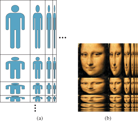
Figure 17.5: (a) A MIP map, schematically. An n×k image is stored in the upper-left corner; to its right is an n × k/2 version of the image, then an n × k/4 version, etc.; below it is an n/2×k image, then an n/4×k image etc. The remaining quadrant is filled in with versions of the image that are condensed both in row size and column size. The recursion stops when the image is reduced to a single pixel. (b) A MIP map for a real image.
The “shrinking” process used to reduce the number of columns by a factor of two is very simple; pairs of adjacent columns are averaged, as shown in Listing 17.1. Analogous code is used to halve the number of rows. The process is repeated, for both rows and columns, until we reach a 1 × 1 image as shown in Figure 17.5.
Listing 17.1: One stage of column reduction for MIP mapping.
1 foreach row of image {
2 for(int c = 0; c < number of columns/2; c++){
3 output[row,c] = (input[row, 2*c] + input[row, 2*c+1])/2;
4 }
5 }
In Chapter 19 you’ll learn the techniques necessary to analyze the MIP-mapping process and determine its limitations. But for now, let’s simply consider the problem of how to MIP-map an image with more than color data. Suppose we have an image, I, storing R-, G-, B-, and α-values (the color values have not been premultiplied by α). The recipe for MIP mapping tells us to average adjacent pairs of colors, but is that the right thing to do when α-values are present as well? Suppose, for instance, that we have a red pixel, with opacity 0, next to a blue pixel of opacity 1. Surely the correct “combined” pixel is blue, with opacity .5. In fact, considering the adjacent pixels as contributing to a single “wide pixel,” we can suppose that we have a left subpixel with colors (RL, GL, BL) and opacity αL, and a right subpixel with subscripts “R” on each item. The left subpixel’s opacity can contribute at most 50% opacity to the wide pixel; the same goes for the right one. Hence the opacity for the wide pixel should be
What about the color of the wide pixel, though? As the red and blue example shows, opacity must be taken into account in the blending process. In fact, the resultant color should be
Thus, we see that even for MIP mapping, it’s natural to use premultiplied α-values for the colors. For further detail on the relationship between MIP mapping and α-values, see McGuire and Stone [MS97].
MIP mapping of other image characteristics such as depth or object ID is more problematic; there’s no clear correct answer.
17.7. Discussion and Further Reading
While our use of images in graphics is primarily in rendering, images themselves have long been a subject of study in their own right, in the field known as image processing. With the advent of image-based rendering (the synthesis of new views of a scene from one or more photographs or renderings of previous views), certain problems arose, such as “What pixel values should I fill in for the parts of the scene that weren’t visible in the previous view, but are in this one?” If it’s a matter of just a pixel or two, filling in with colors from neighboring pixels is good enough to fool the eye, but for larger regions, hole filling is a serious (although obviously underdetermined) problem. Problems of hole filling, combining multiple blurred images to create an unblurred image, compositing multiple images when no a priori masks are known, etc., are at the heart of the emerging field of computational photography. Other aspects of computational photography are the development of cameras with coded apertures (complex masks inside the lens assembly of a camera), and of computational cameras, in which processing built into the camera can adjust the image-acquisition process. Information on Laplace image fill that we provide on this book’s website gives just a slight notion of the power of these techniques.
There’s no clear dividing line between “images” and “rectangular arrays of values.” Organizing graphics-related data in rectangular arrays is powerful because once it’s in this form, any kind of per-cell operation can be applied. But there are even more general things that fit into a broad definition of “image,” and you should open your mind to further possibilities. For instance, we often store samples, many per pixel area, which are then used to compute a pixel value. We’ll see this when we discuss rendering, where we often shoot multiple rays near a pixel center and average the results to get a pixel value. These multiple values are, for practical reasons, often taken at fixed locations around the pixel center, making it easy to compare them, but they need not be. It’s essential, of course, to record the semantics of the samples, just as we earlier suggested recording the semantics of the pixel values. Images containing these multiple values are generally not meant for display—instead, they provide a spatial organization of information that can be converted to a form useful for display or other reuse of the data.
Arrays of samples which are to be combined into values for display require that the combination process must itself be made explicit. In rendering, the “measurement equation,” discussed in Section 29.4.1, makes this explicit.
The notion of coverage, or alpha value, as developed by Porter and Duff, has become nearly universal. At the same time, it has been extended somewhat. Adobe’s PDF format [Ado08], for instance, defines for each object both an “opacity” and a “shape” property for each point. A shape value of 0.0 means that the point is outside the object, and 1.0 means it’s inside. A value like 0.5 is used to indicate that the point is on the edge of a “soft-edged” object. The product of the shape and opacity values, on the other hand, corresponds to the alpha value we’ve described in this chapter. These two values can then be used to define quite complex compositing operations.
17.8. Exercises
Exercise 17.1: The blend operation can be described by what happens to a point in a pixel that’s in neither the opaque part of U nor the opaque part of V, in just U, in just V, or in both. Give such a description. Is the U-and-V part of the composition consistent with our assumptions about the distribution of the opaque parts of each individual pixel?
Exercise 17.2: Suppose you needed to store images that contained many large regions of constant color. Think of a lossless way to compress such images for more compact storage.
Exercise 17.3: Implement the checkerboard-selection lossy compression scheme described in this chapter; try it on several images and describe the artifacts that you notice in the redisplayed images.
Exercise 17.4: Our description of MIP maps was informal. Suppose that M is a MIP map of some image, I. It’s easy to label subparts of M: We let Ipq be the subimage that is I, shrunk by 2p in rows and by 2q in columns. Thus, the upper-left corner of M, which is a copy of the original image, is I00; the half-as-wide image to its right is I01; the half-as-tall image below I00 is I10, etc. If you consider the subimage of I consisting of all parts Ipq where p ≥ 1, it’s evidently a MIP map for I10; a similar statement holds for the set of parts where q ≥ 1: It’s the MIP map for I01. Use this idea to formulate a recursive definition of the MIP map of an image I. You may assume that I has a width and height that are powers of two.
Exercise 17.5: MIP mapping is often performed as a preprocess on an image, with the MIP map itself being used many times. The preprocessing cost is therefore relatively unimportant. Nonetheless, for large images, especially those so large that they cannot fit in memory, it can be worth being efficient. Assume that the source image I and the MIP map M are both too large to fit in memory, and that they are stored in row-major order (i.e., that I[0, 0], I[0, 1], I[0, 2], ... are adjacent in memory), and that each time you access a new row it incurs a substantial cost, while accessing elements in a single row is relatively inexpensive. How would you generate a MIP map efficiently under these conditions?