
Chapter 30. Probability and Monte Carlo Integration
30.1. Introduction
In preparation for studying rendering techniques, we now discuss Monte Carlo integration. We start with a rapid review of ideas from discrete probability theory, and then generalize to continua like the real line or the unit sphere. We apply these notions to describe how to generate random samples from various sets. We then introduce Monte Carlo integration, treating all the basic ideas through the integration of a function on an interval [a, b], where the ideas are easiest to understand. We then show how these ideas apply to integration on a hemisphere or sphere, and hence how they are used to find reflected radiance via the reflectance equation, for instance.
30.2. Numerical Integration
We’ll start with a high-level overview of the use of randomization in numerical integration. Sometimes we need to integrate functions where computing antiderivatives is impossible or impractical. For instance, the integrand in the reflectance equation might not be described by an algebraic equation at all. In these cases, numerical methods often are the only workable solution. Numerical methods fall into two categories: deterministic and randomized. Here’s a quick comparison of the two.
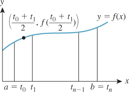
A typical deterministic method (see Figure 30.1) for integrating a function f over an interval [a, b] is to take n + 1 equally spaced points in the interval [a, b], t0 = a, t1= a + ![]() , ..., tn = b, evaluate f at the midpoint
, ..., tn = b, evaluate f at the midpoint ![]() of each of the intervals these points define, sum up the results, and multiply by
of each of the intervals these points define, sum up the results, and multiply by ![]() , the width of each interval. For sufficiently continuous functions f, as n increases this will converge to the correct value. Similar methods for surface integrals, which divide the surface into small rectangles, also work. Press et al. [Pre95] describe these and more sophisticated deterministic methods.
, the width of each interval. For sufficiently continuous functions f, as n increases this will converge to the correct value. Similar methods for surface integrals, which divide the surface into small rectangles, also work. Press et al. [Pre95] describe these and more sophisticated deterministic methods.
A probabilistic or Monte Carlo method for computing, or more precisely, for estimating the integral of f over the interval [a, b], is this: Let X1, ..., Xn be randomly chosen points in the interval [a, b]. Then ![]() is a random value whose average (over many different choices of X1, ..., Xn) is the integral
is a random value whose average (over many different choices of X1, ..., Xn) is the integral ![]() . To implement this we use a random number generator to generate n points xi in the interval [a, b], evaluate f at each, average the results, and multiply by b – a. This gives an estimate of the integral, as shown in Figure 30.2. Of course, each time we compute such an estimate we’ll get a different value. The variance in these values depends on the shape of the function f. If we generate the random points xi nonuniformly, we must slightly alter the formula. But in using a nonuniform distribution of points we gain an enormous advantage: By making our nonuniform distribution favor points xi where f (x) is large, we can drastically reduce the variance of our estimate. This nonuniform sampling approach is called importance sampling. Figure 30.3 shows an example.
. To implement this we use a random number generator to generate n points xi in the interval [a, b], evaluate f at each, average the results, and multiply by b – a. This gives an estimate of the integral, as shown in Figure 30.2. Of course, each time we compute such an estimate we’ll get a different value. The variance in these values depends on the shape of the function f. If we generate the random points xi nonuniformly, we must slightly alter the formula. But in using a nonuniform distribution of points we gain an enormous advantage: By making our nonuniform distribution favor points xi where f (x) is large, we can drastically reduce the variance of our estimate. This nonuniform sampling approach is called importance sampling. Figure 30.3 shows an example.
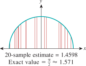
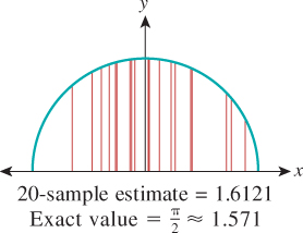
Figure 30.3: Estimating the same integral, again with 20 samples, but preferentially selecting samples near x = 0, and using appropriate weighting, gives a better approximation.
We can integrate a function f over a surface region R by an analogous method. We choose points uniformly randomly on R, average the values of f at these points, and multiply by the area of the region. Or we can generate points nonuniformly, and compute a weighted average, again multiplied by the region’s area, generalizing importance sampling. Our main application of numerical integration is when R is either the sphere or the outward-facing hemisphere at some surface point P where we’re trying to compute the scattered light (i.e., trying to evaluate the integral in the reflectance equation). We’ll return to this application at the end of the chapter.
Randomized integration techniques form part of the working tools of anyone studying rendering, and much of the rest of graphics. Press et al. [Pre95] is a solid first reference for ideas beyond those discussed in this chapter.
30.3. Random Variables and Randomized Algorithms
Because the major shift in rendering methods over the past several decades was from deterministic to randomized, we’ll be discussing randomized approaches to solving the rendering equation. To do so means using random variables, expectation, and variance, all of which we assume you have encountered in some form in the past. To establish notation, and prepare for the continuum and mixed-probability cases, we review discrete probability here. The approach we take may seem a little unusual. That’s because our goal is not to analyze some probabilistic phenomenon that already exists (e.g., the chance of rainfall in Boston tomorrow, given that it’s already been raining for two days), but rather to construct probabilistic situations in which something computable, like expected value, turns out to have the same value as some integral (like the reflectance integral) that we care about. That leads to emphasis on some things that are largely downplayed in introductory probability courses.
We often find that for our students, the connection between formal probability theory and programs that implement probabilistic ideas is unclear, and so we discuss this connection as well.
Those familiar with these concepts can skip forward to Section 30.3.8.
30.3.1. Discrete Probability and Its Relationship to Programs
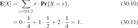
A discrete probability space is a nonempty finite1 set S together with a real-valued function p : S ![]() R with two properties.
R with two properties.
1. Countably infinite sets such as the integers are often included in the study of discrete probability, but we’ll have no need for them, and restrict ourselves to the finite case.
1. For every s ε S, we have p(s) ≥ 0, and
2. ![]() .
.
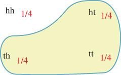
The first property is called non-negativity, and the second is called normality. The function p is called the probability mass function, and p(s) is the probability mass for s (or, informally, the probability of s). The intuition is that S represents a set of outcomes of some experiment, and p(s) is the probability of outcome s. For example, S might be the set of four strings hh, ht, th, tt, representing the heads-or-tails status of tossing a coin twice (see Figure 30.4). If the coin is fair, we associate probability ![]() to each outcome.
to each outcome.
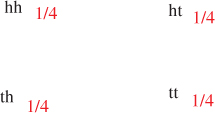
Figure 30.4: A four-element probability space, with uniform probabilities, shown as fractions in red.
Explain why, in a discrete probability space (S, p), we have 0 ≤ p(s) ≤ 1 for every s ε S. The first inequality follows from the first defining property of p. What about the second?
An event is a subset of a probability space. The probability of an event (see Figure 30.5) is the sum of the probability masses of the elements of the event, that is,
Prove that if E1 and E2 are events in the finite probability space S, and E1 ![]() E2 =
E2 = ![]() , then Pr{E1
, then Pr{E1 ![]() E2} = Pr{E1} + Pr{E2}. This generalizes, by induction, to show that for any finite set of mutually disjoint events,
E2} = Pr{E1} + Pr{E2}. This generalizes, by induction, to show that for any finite set of mutually disjoint events, ![]() . One of the axioms of probability theory is that this relation holds even for an infinite, but countable, collection of disjoint events when we’re working with continua, like [0, 1] or R, rather than a discrete probability space.
. One of the axioms of probability theory is that this relation holds even for an infinite, but countable, collection of disjoint events when we’re working with continua, like [0, 1] or R, rather than a discrete probability space.
A random variable is a function, usually denoted by a capital letter, from a probability space to the real numbers:
The terminology is both suggestive and misleading. The function X is not a variable; it’s a real-valued function. It’s not random, either: X(s) is a single real number for any outcome s ε S. On the other hand, X serves as a model for something random. To give a concrete example, consider the four-element probability space described earlier. There’s a random variable X defined on that space by the notion “How many heads came up?” or, more formally, “How many hs does the string contain?” To be explicit, we can define the random variable X by
This function takes on real values (either 0, 1, or 2), and it’s defined on the set S; hence, it’s a random variable. As in this example, we’ll use the letter X to denote nearly every random variable in this chapter.
A random variable can be used to define events. For example, the set of outcomes s for which X(s) = 1, that is,
is an event with probability ![]() . We write this Pr{X = 1} =
. We write this Pr{X = 1} = ![]() , that is, we use the predicate X = 1 as a shorthand for the event defined by that predicate.
, that is, we use the predicate X = 1 as a shorthand for the event defined by that predicate.
Let’s look at a piece of code for simulating the experiment represented by the formalities above:
1 headcount = 0
2 if (randb()): // first coin flip
3 headcount++
4 if (randb()): // second coin flip
5 headcount++
6
7 return headcount
Here we’re assuming the existence of a randb() procedure that returns a boolean, which is true half the time.
How is this simulation related to the formal probability theory? After all, when we run the program the returned value will be either 0, 1, or 2, not some mix of these. (If we run it a second time, we may get a different value, of course.)
The relationship between the program and the abstraction is this: Imagine the set S of all possible executions of the program, declaring two executions to be the same if the values returned by randb are pairwise identical. This means that there are four possible program executions, in which the two randb() invocations return TT, TF, FT, and FF. Our belief and experience is that these four executions are equally likely, that is, each occurs just about one-quarter of the time when we run the program many times.
The analogy is now clear: The set of possible program executions, with associated probabilities, is a probability space; the variables in the program that depend on randb invocations are random variables. This is a quite clever piece of mathematical modeling of computation. You should be certain that you understand it.
![]() There’s nice formalism in which a procedure that invokes
There’s nice formalism in which a procedure that invokes randb-like functions is replaced by one with an extra argument, which is a long string of bits; these bits are used instead of randb calls. This revised procedure is deterministic; it becomes randomized only when we invoke it with a sequence of random bits. In this formalism, the probability space is the set of all possible bit strings that are provided as the extra argument.
30.3.2. Expected Value
The expectation or expected value or mean of a random variable X on a finite probability space S is defined as
In the case of our “counting heads in a coin-flip” experiment, the expectation is
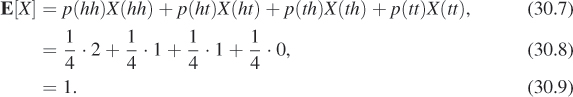
If we in fact run the coin-flipping program many times, we’ll sometimes see a heads count of 0; sometimes 1; and sometimes 2. The average number of heads, over many executions of the program, will be about 1.
We can rewrite the expectation in Equation 30.7 by asking, for each possible value taken on by X (i.e., 0, 1, and 2), what fraction of the items in S correspond to that value. For the value 1, we have X(ht) = 1 and X(th) = 1, so two of the four items in S, in other words, half, correspond to the value 1. We then sum these fractions times the associated values, and thus compute
This latter form is used in many applications of probability, because it depends only on the values of X and the associated probabilities, and the probability space S does not appear directly. In our applications, however, this form will not appear again.
Nonetheless, the function r ![]() Pr {X = r}, and its generalization in the continuum case, is of substantial interest to us. Note that it’s defined on the codomain of X, not the domain. And for each codomain value r, it tells us (if we’re thinking of X informally as “producing a random output”) the probability that X will produce the output r. This function is called the probability mass function (or pmf) for the random variable X, and is denoted pX.
Pr {X = r}, and its generalization in the continuum case, is of substantial interest to us. Note that it’s defined on the codomain of X, not the domain. And for each codomain value r, it tells us (if we’re thinking of X informally as “producing a random output”) the probability that X will produce the output r. This function is called the probability mass function (or pmf) for the random variable X, and is denoted pX.
One reason the pmf is interesting is that it can be generalized to apply to a function Y : S ![]() T, sending our probability space to any finite set T, not just the real numbers. For such a function, we define
T, sending our probability space to any finite set T, not just the real numbers. For such a function, we define
This function, pY, is a probability mass function on T so that (T, pY) becomes a probability space.
(a) How do we know that pY is a probability mass function, that is, it satisfies the two requirements of non-negativity and normality?
(b) If E ![]() T is an event, show that Equation 30.12 implies that the probability of the event E in the space (T, pY) is given by PrT{E} = PrS{Y–1(E)}. (Here Y1(E) denotes the set of all points s ε S such that Y(s) ε E.)
T is an event, show that Equation 30.12 implies that the probability of the event E in the space (T, pY) is given by PrT{E} = PrS{Y–1(E)}. (Here Y1(E) denotes the set of all points s ε S such that Y(s) ε E.)
We’ve now used the term “probability mass function” in two different ways: When we spoke of a probability space (S, p), we called p the probability mass function. But we’ve also described the pmf for a random variable X : S ![]() R, or even for a function Y : S
R, or even for a function Y : S ![]() T into an arbitrary set. We’ll now show that these uses are consistent. Consider the identity function I : S
T into an arbitrary set. We’ll now show that these uses are consistent. Consider the identity function I : S ![]() S : s
S : s ![]() s. By Equation 30.12, we have
s. By Equation 30.12, we have
For a fixed element t ε S, what is the event I = t? It’s the event
The probability of this event is just the sum of the probability masses for all outcomes in the event, that is, p(t). Thus, the probability mass function for the identity map is the same thing as the probability mass function p for the probability space itself.
Functions like Y that send a probability space to some set T rather than R are sometimes still called random variables. In the case we’re most interested in, Y will send the unit square to the unit sphere or upper hemisphere, and we’ll use the terminology “random point.” We’ll use the letter Y to denote random-point functions, just as we use X for all the random variables in the chapter.
We conclude with one last bit of terminology. The function pY, whether Y is a random variable or a map from S to some arbitrary set T, is called the distribution of Y; we say that Y is distributed according to pY. This suggestive terminology is useful when we’re thinking of things like student scores on a test, where it’s common to say, “The scores were distributed around a mean of 82.” In this case, the underlying probability space S is the set of students, with a uniform probability distribution on S, and the test score is a random variable from students to R. You’ll often see the notation X ~ f to mean “X is a random variable with distribution f,” that is, with pX = f.
30.3.3. Properties of Expected Value, and Related Terms
The expected value of a random variable X is a constant; it’s often denoted ![]() . Note that
. Note that ![]() can also be regarded as a constant function on S, and hence be treated as a random variable as well.
can also be regarded as a constant function on S, and hence be treated as a random variable as well.
Expectation has two properties that we’ll use frequently: E[X + Y] = E[X] + E[Y], and E[cX] = cE[x] for any real number c. In short, expectation is linear.
Expectation and variance (the latter which we’ll encounter in a moment) are higher-order functions: Their arguments are not numbers or points, but actual functions—in particular, random variables.
When we write E[X + Y], we mean the expectation of the sum of the two random variables X and Y, that is, the function s ![]() X(s) + Y(s). This means that when we write X + X, we mean the function s
X(s) + Y(s). This means that when we write X + X, we mean the function s ![]() X(s) + X(s). If X happens to correspond to a piece of code that looks like
X(s) + X(s). If X happens to correspond to a piece of code that looks like return randb(...), then you cannot implement X + X by X() + X(): The two invocations of the random number generator may produce different values!
In general, when you look at a program with randb in it, your analysis of the program will involve a probability space with 2k elements, where k is the number of times randb is invoked; each element will have equal probability mass. The same will be true when we look at rand: Any two numbers between 0 and 1 will be equally likely to be the output of any invocation of rand. We call randb a uniform random variable, because all of its outputs are equally likely.
Note that if randb is invoked a variable number of times in the program, then some elements of the program’s probability space will have greater probability than others.
Suppose we modify our coin-flipping program to only flip twice if the first coin came up heads, as in Listing 30.1. Describe a probability space for this code, and compute the expected value of the random variable headcount.
Listing 30.1: A program in which randb is invoked either once or twice.
1 headcount = 0
2 if (randb()): // first coin flip
3 headcount++
4 if (randb()): // second coin flip
5 headcount++
6 return headcount
The values taken on by a random variable X may be clustered around the mean ![]() , or widely dispersed. This dispersion is measured by the variance, the mean-square average of X(s) –
, or widely dispersed. This dispersion is measured by the variance, the mean-square average of X(s) –![]() . Formally, the variance is
. Formally, the variance is
which can be simplified (see Exercise 30.9) to E[X2] – E[X]2.
The units of variance are the units of X, squared; the square root of the variance (known as the standard deviation) has the same units as X, and sometimes makes better intuitive sense. As a useful rule of thumb, three-fourths of the values of X lie within two standard deviations of ![]() .
.
Variance is not linear, but has the property that Var[cX + d] = c2Var[X] for any real numbers c and d.
The random variables X and Y are called independent if
for every x and y in R. For instance, in the experiment where we flip an unbiased coin twice, if X is the number of heads that show up on the first coin flip (either 0 or 1), and Y is the number of heads that show up on the second, then our experience tells us that X and Y are independent, that is, the probability of two heads in a row is ![]() . On the other hand, the variables X and X are distinctly not independent. We’ll generally assume that any two values produced by calls to
. On the other hand, the variables X and X are distinctly not independent. We’ll generally assume that any two values produced by calls to randb or rand or other such functions correspond to independent random variables.
The important properties for independent random variables are
• E[XY] = E[X]E[Y]
• Var[X + Y] = Var[X] + Var[Y]
Returning to the coin-flip experiment and the associated program, we implemented the two random variables via calls to a single random-number-generating routine, randb. We call these random variables samples from the distribution in which heads and tails have equal probability. The idea is that randb can be thought of as producing a long list of random zeroes and ones, each equally likely, and we’ve simply grabbed a couple of these.
Together, these two samples are therefore independent, and, because they came from the same distribution, identically distributed. Such random variables occur often, and we refer to them as independent identically distributed or iid random variables or samples.
30.3.4. Continuum Probability
The entire discrete-probability framework can be extended by analogy to countably infinite sets, which requires some care because we have to talk about sums of infinite series, and worry about convergence. That particular case isn’t of much interest in graphics, but the study of probability on uncountably infinite domains like the unit interval, or the unit sphere, comes up repeatedly. We’ll refer to such a domain, on which you know how to compute integrals, as a continuum, and speak of continuum probability as contrasted with the discrete probability discussed earlier. Some books use the term continuous probability for this situation, but since we’ll want to be able to discuss continuous and discontinuous functions, we prefer “continuum.” In the continuum case, we’ll analyze programs that contain rand (which returns random real numbers between 0 and 1, with every number being just as likely as every other number) rather than randb. There are three difficulties.
1. The procedure rand doesn’t really produce real numbers in [0, 1]; it produces floating-point representations of a tiny subset of them.
2. ![]() Certain aspects of the analysis involve mathematical subtleties like measurability.
Certain aspects of the analysis involve mathematical subtleties like measurability.
3. Our probability space will now be infinite, and we’ll need to talk about probability density rather than probability mass.
We’ll mostly ignore difficulties 1 and 2, on the grounds that they have little impact in the practical applications we make. Difficulty 3, however, matters quite a lot.
Let’s look at another sample program as motivation. To make the code as readable as possible, we’ll avoid the use of rand and instead write uniform(a, b) to indicate a procedure that produces a random real number between a and b, with each output being equally probable. This is typically implemented with a + (b-a)*rand().
1 u = uniform(0,1); // a random real between 0 and 1
2 w = ![]()
3 return w
On the next several pages, we’ll describe the sample space associated with this program, the notion of probability density, and the definitions of random variable and expected value, and will eventually compute the expected value of w.
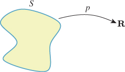
First, for this continuum situation, a probability space is a pair (S, p) consisting of a set S, such as the real line, the unit interval, the unit square, the upper hemisphere, the whole sphere, etc., on which integration is defined, and a probability density function, or just densityp : S ![]() R (see Figure 30.6), with two properties:
R (see Figure 30.6), with two properties:
• Non-negativity: For all s ε S, p(s) ≥ 0
• Normality: ∫S p = 1
The second property means that when p is integrated over all of S, the result is 1, whether S is something one-dimensional like the interval [a, b], in which case the normality condition would be written ![]() , or something two-dimensional, like the unit square, in which case we’d write
, or something two-dimensional, like the unit square, in which case we’d write
For the most part our probability spaces will be things like the interval or the sphere, which have the property that when we integrate the constant function 1 over them, the result is some finite value, which we’ll call the size of S, and denote size(S). In these cases, the associated density will usually be the constant function with value 1/size(S), called a uniform density. Note that there is no uniform density for the real line, however.
In the discrete case, the normality condition involved a sum; in the continuum case, it involves an integral. You might be tempted to think of the probability density as just like the probability mass in the discrete case, but they’re quite different, as the next inline exercise shows. The proper interpretation is that the density represents probability per unit size. Thus, in cases where we have units, probability and probability density differ by the units of size (i.e., length, area, or volume).
Let S = [0, 1] and p(x) = 2x. Show that (S, p) is a probability space by checking the two conditions on p. Observe that p(1) = 2, so a probability density may have values greater than 1, even though probability masses are never greater than 1.
To return to our program, the set of all possible executions of the program is infinite:2 In fact, there’s one execution for every real number between 0 and 1. So we can say that our probability space is S = [0, 1], the unit interval. And since we regard each possible value of uniform(0,1) as equally likely, we associate to S the uniform density defined by p(x) = 1 for all x ε [0, 1].
2. We’re pretending that our random number generator returns real numbers, rather than floating-point representations of them.
Just as in the discrete case, a random variable is a function X from S to R, and an event is a subset of S, but we’ll mostly restrict our attention to events of the form a ≤ X ≤ b, where X is some random variable.
![]() To be honest, not every subset of S is an event; only the “measurable” ones. But it’s essentially impossible to write down a non-measurable set, and certainly not possible to encounter one while performing computations on an ordinary computer, so we’ll ignore this subtlety. If you like, you may consider events to be restricted to things like intervals or rectangles, or other similarly nice sets over which you know how to integrate.
To be honest, not every subset of S is an event; only the “measurable” ones. But it’s essentially impossible to write down a non-measurable set, and certainly not possible to encounter one while performing computations on an ordinary computer, so we’ll ignore this subtlety. If you like, you may consider events to be restricted to things like intervals or rectangles, or other similarly nice sets over which you know how to integrate.
The probability of an event E in a probability space (S, p) is the integral of p over E, just as in the discrete space the probability of an event is the sum of the probability masses of the points in the event.
The expected value of a random variable X on a probability space (S, p) is defined to be
As in the discrete case, expectation is linear.
(a) In the special case where S is a space with a uniform density, show that the expectation of the random variable X is just ![]() .
.
(b) What is the expectation of a random variable Z on the interval [a, b] with uniform density?
We’ll now apply the notion of expectation to the example code. The variable u in the program corresponds to a random variable U on the interval [0, 1]. Similarly, the variable w in the program corresponds to a random variable W = ![]() . The expected value of W is, according to the definition,
. The expected value of W is, according to the definition,
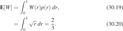
This should match your intuition: The variable U is uniformly distributed on [0, 1], so its expected value is ![]() . But for any number 0 < u < 1, we have u <
. But for any number 0 < u < 1, we have u < ![]() , so the average square root of any number should be bigger than the average number, that is, we anticipate that the expected value of W will be somewhat larger than
, so the average square root of any number should be bigger than the average number, that is, we anticipate that the expected value of W will be somewhat larger than ![]() .
.
30.3.5. Probability Density Functions
In analogy with the probability mass function for a random variable on a discrete space described in Section 30.3.2, we’ll now formulate the corresponding notion for a random variable on a continuum.
It often happens that for a random variable X, and the special class of events of the form a ≤ X ≤ b (i.e., the set {s : a ≤ X(s) ≤ b}), there’s a function pX, called the probability density function (pdf) or density or distribution for X, with the property that
For the time being, we’ll consider only random variables that have a pdf.
The intuition for pX, for a random variable X, is that for small values of Δ, the number pX(a)Δ is approximately the probability that X lies in an interval of size Δ, centered at a, or [a – Δ/2, a +Δ/2], with the approximation being better and better as Δ ![]() 0.
0.
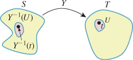
Just as in the discrete case, if S is a continuum probability space with associated density p and
we can use Y to define a probability density on T (see Figure 30.7). We’ll restrict our attention to the special case where Y is an invertible function, although we’ll apply the results to cases where Y is “almost invertible,” like the latitude-longitude parameterization of the sphere, where the noninvertibility is restricted to a set whose “size” is zero. In the case of the spherical parameterization, if we ignore all points of the international dateline, the parameterization is 1-1, and the dateline itself has size zero (where “size,” for a surface, means “area”).
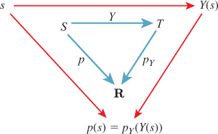
Figure 30.7: The density pY is defined so that starting from a point s ε S, you get the same result no matter which way you traverse the arrows, that is, p(s) = pY(Y(s)).
Our definition closely follows the discrete case:
Returning to the example program, the variable U has as its pdf the function
This evidently integrates to 1 on the whole interval.
For any particular number, like r = 0.3, the probability that U = r is ![]() . Intuitively, if we’re picking a random number between 0 and 1, the probability of picking any particular number ends up being zero. Despite this, we do pick some number. This is a situation where the probability of a union of disjoint events (the events being “pick 0.134,” “pick π/13,” and infinitely many other similar events) is not the sum of the individual probabilities. Thus, when we shift from finite sets to infinite ones, some of our intuition about probability turns out to be mistaken.
. Intuitively, if we’re picking a random number between 0 and 1, the probability of picking any particular number ends up being zero. Despite this, we do pick some number. This is a situation where the probability of a union of disjoint events (the events being “pick 0.134,” “pick π/13,” and infinitely many other similar events) is not the sum of the individual probabilities. Thus, when we shift from finite sets to infinite ones, some of our intuition about probability turns out to be mistaken.
The pdf for W is not so obvious. Evidently, values near 0 occur less often as outputs of W than do those near 1, but what’s the exact pattern? The answer is obviously not that it’s the square root of the pdf for U. We seek a function pW with the property that
In the left-hand side of this equation is the event that a ≤ W ≤ b; let’s rewrite this:
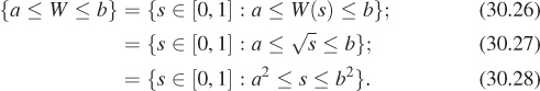
The probability of that last event is b2 –a2. (Why?) So we need to find a function pW with the property that for any a, b ε [0, 1],
A little calculus shows that pW (r) = 2r (see Exercise 30.4).
The notion of a random variable can be generalized to that of a random point. If S is a probability space, and Y : S ![]() T is a mapping to another space rather than the reals, then we call Y a “random point” rather than a random variable. The notion of a probability density applies here as well, but rather than just looking at an interval [a, b]
T is a mapping to another space rather than the reals, then we call Y a “random point” rather than a random variable. The notion of a probability density applies here as well, but rather than just looking at an interval [a, b] ![]() R, we must now consider any set U
R, we must now consider any set U ![]() T; we’ll say that pY is a pdf for the random variable Y if, for every (measurable) subset U
T; we’ll say that pY is a pdf for the random variable Y if, for every (measurable) subset U ![]() T, we have
T, we have
In fact, it’s usually fairly easy to compute pY if we know the mapping Y by an argument completely analogous to the one used to find pW.
In the special case where S has a uniform probability density (see Figure 30.8), the probability of Y ε U is just the probability of the set Y–1(U) ![]() S, which is the size of Y1(U) divided by the size of S.
S, which is the size of Y1(U) divided by the size of S.
If we assume that pY is continuous, then we can compute pY directly. Consider the case of a very small neighborhood U of some point t ε T; then the right-hand side is given by
On the other hand, the left-hand side is given by a ratio of sizes as described above, so
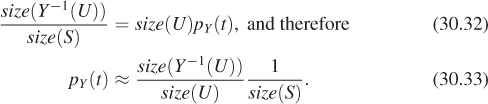
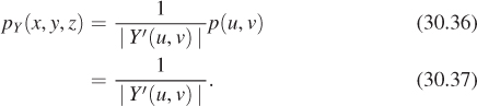
The first factor in this expression is just an approximation of the change of area for Y–1, which is given by the Jacobian of Y–1 at t. So in the limit, as U shrinks to a smaller and smaller neighborhood of Y(t), we get
As in the discrete case, we can use pY as a probability density for the space T, or we can simply use it as the pdf for the random point Y.
And once again, if ![]() : S
: S ![]() S : s
S : s ![]() s is the identity map, then p
s is the identity map, then p![]() = p, so the two notions of density—the probability density used in defining a continuum probability space, and the probability density of a random variable on that space—are in fact consistent.
= p, so the two notions of density—the probability density used in defining a continuum probability space, and the probability density of a random variable on that space—are in fact consistent.
Finally, we will again use the notation X ~ f to mean “X is a random variable distributed according to f” which in the continuum case means that pX = f. There is one standard distribution that we’ll use repeatedly, U(a, b), which is the uniform distribution on [a, b], or the constant function ![]() . You’ll often see this in forms like “Suppose X, Y ~ U(0, π) are two uniform random variables ...”
. You’ll often see this in forms like “Suppose X, Y ~ U(0, π) are two uniform random variables ...”
30.3.6. Application to the Sphere
Let’s apply the ideas of the previous section to the longitude-colatitude parameterization of S2, namely,
We’ll start with the uniform probability density p on [0, 1] × [0, 1], or p(u, v) = 1 for all u, v. For notational convenience, we’ll write (x, y, z) = Y(u, v).
We have the intuitive sense that if we pick points uniformly randomly in the unit square and use f to convert them to points on the unit sphere, they’ll be clustered near the poles. (If you doubt this, you should write a little program to verify it.) This means that the induced probability density on T will not be uniform.
The preceding section shows that
But the change-of-area factor (see Figure 30.9) for Y (which is slightly messy to compute) turns out to be
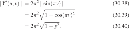
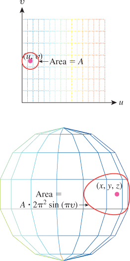
Figure 30.9: A small area A in the domain of the spherical parameterization gets multiplied by 2π2 sin(πv).
And hence,
Thus, the probability of sampling a point in a small disk of area A centered on the sphere point (x, y, z) is approximately ![]() .
.
30.3.7. A Simple Example
If we start with the uniformly distributed random variable U on [0, 1] × [0, 1] and want a uniformly distributed variable V on, say, [0, 2π] × [0, 1], it seems obvious to define ![]() . The density for U is the function
. The density for U is the function
That makes the density for V be the function
(Quick proof: V is evidently uniformly distributed, and hence its pdf is a constant. The integral of that constant over the domain must be 1, so the constant is ![]() .)
.)
1 x = uniform(0, 1);
2 y = uniform(0, 1); // U = (x, y)
3 x' = 2 * π * x;
4 y' = y; // V= (x’, y’)
5 return (x', y')
There’s no mention of the pdf in the code, but it matters nonetheless when we want to analyze the code.
30.3.8. Application to Scattering
The ability to easily draw samples from a distribution (i.e., to produce many independent random variables all having the same specified pdf) will be critical in rendering. In estimating the reflectance integral, we sometimes want to pick a random direction ω in the positive hemisphere with probability density proportional to the bidirectional reflectance distribution function (BRDF), with the first argument held constant at the incoming direction, that is, the function ω ![]() fr(ωi,ω). (Notice that this function is not in general a probability density on the hemisphere: Its integral is not 1.) Unfortunately, sampling in proportion to a general function on the hemisphere is not often easy.
fr(ωi,ω). (Notice that this function is not in general a probability density on the hemisphere: Its integral is not 1.) Unfortunately, sampling in proportion to a general function on the hemisphere is not often easy.
We now examine two examples where such direct sampling is possible.
Example 1: The Lambertian BRDF. We need to choose a direction on the hemisphere uniformly at random (i.e., the probability that the direction lies in any solid angle ![]() is proportional to the measure of Ω.) In fact, since the total area of the hemisphere is 2π, we need the probability that the direction lies in a solid angle Ω to be exactly
is proportional to the measure of Ω.) In fact, since the total area of the hemisphere is 2π, we need the probability that the direction lies in a solid angle Ω to be exactly ![]() .
.
Fortunately, as we saw in Section 26.6.4, the map
from the unit cylinder around the y-axis to the unit sphere is area-preserving (although it’s not length- or angle-preserving). By restricting our attention to the half-cylinder
we get an area-preserving map from H to ![]() . And the map
. And the map
multiplies areas by exactly 2π, as you can check by computing its Jacobian. So the composition Y = g ° f of the two gives us a map from the unit square to ![]() that multiplies areas by 2π. The density for Y is therefore the constant function
that multiplies areas by 2π. The density for Y is therefore the constant function ![]() on
on ![]() .
.
In the program shown in Listing 30.2, the returned point is a random point on the hemisphere with density ![]() .
.
Listing 30.2: Producing a uniformly distributed random sample on a hemisphere.
1 Point3 randhemi()
2 u = uniform(0, 1)
3 v = uniform(0, 1)
4 r = sqrt(1 - y*y)
5 return Point3(r cos(2πu), y, r sin(2πu));
Example 2: Cosine-weighted sampling on a hemisphere. Now suppose that we want to sample from a hemisphere, but we want the probability of picking a point in the neighborhood of ω to be proportional to ω · n, where n = [0 1 0]T is the unit normal to the xz-plane that bounds the hemisphere. If we write ω = [x y z], then ω · n is simply y.
The function (x, y, z) ![]() y is not a probability density on the hemisphere y ≥ 0, because its integral is π rather than 1.0. Thus,
y is not a probability density on the hemisphere y ≥ 0, because its integral is π rather than 1.0. Thus, ![]() is a pdf. We’d now like to sample from this pdf (i.e., we’d like to create a random-point Y whose distribution is this pdf). Because of the area-preserving property of the radial projection map, we can instead choose a random point on the half-cylinder, with density
is a pdf. We’d now like to sample from this pdf (i.e., we’d like to create a random-point Y whose distribution is this pdf). Because of the area-preserving property of the radial projection map, we can instead choose a random point on the half-cylinder, with density ![]() , and then project to the hemisphere.
, and then project to the hemisphere.
Because the density is independent of the angular coordinate on the cylinder, all we need to do is to generate values of y ε [0, 1] whose density is proportional to y. The computation following Equation 30.26 shows that if U is uniformly distributed on [0, 1], then W = ![]() is linearly distributed, that is, the probability density for W at t ε [0, 1] is 2t.
is linearly distributed, that is, the probability density for W at t ε [0, 1] is 2t.
Listing 30.3 shows the resultant code.
Listing 30.3: Producing a cosine-distributed random sample on a hemisphere.
1 Point3 cosRandHemi()
2 θ = uniform(0, 2 * M_PI)
3 s = uniform(0, 1)
4 y = sqrt(s)
5 r = sqrt(1 - y2)
6 return Point3(r cos(θ), y, r sin(θ))
So certain distributions, like the uniform and the cosine-weighted ones, are easy to sample from. More general distributions are often not. When we design reflectance models (i.e., families of BRDFs that can be fit to observed data), one of the criteria, naturally, is goodness of fit: “Is our family rich enough to contain functions that match the observed data decently?” Another criterion is, “Once we fit our data, will we be able to sample from the resultant distributions effectively?” The two criteria are somewhat related, as described by Lawrence et al. [LRR04], who propose a factored BRDF model from which it’s easy to do effective importance sampling.
30.4. Continuum Probability, Continued
We’re now going to talk about ways to estimate the expected value of a continuum random variable, and using these to evaluate integrals. This is important because in rendering, we’re going to want to evaluate the reflectance integral,
for various values of P and ωo. Knowing how to build a random variable whose expected value is exactly this integral will be a big help in this evaluation.
We saw that code that generated a random number uniformly distributed on [0, 1] and took its square root produced a value between 0 and 1 whose expected value was ![]() . This also happens to be the average value of
. This also happens to be the average value of ![]() on that interval. This wasn’t just a coincidence, as the following theorem shows.
on that interval. This wasn’t just a coincidence, as the following theorem shows.
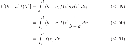
Theorem: If f : [a, b] ![]() R is a real-valued function, and X ~ U(a, b) is a uniform random variable on the interval [a, b], then (b – a)f(X) is a random variable whose expected value is
R is a real-valued function, and X ~ U(a, b) is a uniform random variable on the interval [a, b], then (b – a)f(X) is a random variable whose expected value is
This is a big result! It says that we can use a randomized algorithm to compute the value of an integral, at least if we run the code often enough and average the results. The remainder of this chapter amplifies and improves this result.
The proof of the theorem is simple. The pdf for X is ![]() , so the expected value for (b – a)f(X) is
, so the expected value for (b – a)f(X) is
Listing 30.4 shows the corresponding program.
Listing 30.4: Estimating the integral of the real-valued function f on an interval.
1 integrate1(double *f (double), double a, double b):
2 // estimate the integral of f on [a, b]
3 x = uniform(a, b) // a random real number in [a, b]
4 y = (*f)(x) * (b - a)
5 return y
The value y returned by the program is a random variable that’s an estimate of the integral of f. The average quality of this estimate is measured by the variance of y, which depends on the function f. If f is constant, for example, the estimate is always exactly correct; if f has enormous variations (e.g., ![]() ), then the estimate is highly likely to be very bad. While it’s true that if we run the program many times and average the results, we’ll get something close to the correct value of the integral, any individual run of the program is likely to produce a value that’s very far from the correct value.
), then the estimate is highly likely to be very bad. While it’s true that if we run the program many times and average the results, we’ll get something close to the correct value of the integral, any individual run of the program is likely to produce a value that’s very far from the correct value.
Implement the small program above in your favorite language, and apply it to estimate the average value of a few functions—say, f(x) = 4, f(x) = x2, and f(x) = sin(πx) on the interval [0, 2π].
In general, when we think of a random variable as providing an estimate of some value, low variance is good and high variance is bad.
Let’s now improve our estimation of the integral by taking two iid samples (see Listing 30.5).
Listing 30.5: Estimating the integral of the real-valued function f on an interval, version 2.
1 def integrate2(double *f (double), double a, double b):
2 // estimate the integral of f on [a, b]
3 x1 = uniform(a, b) // random real number in [a, b]
4 x2 = uniform(a, b) // second random real number in [a, b]
5 y = 0.5* ((*f)(x1) + (*f)(x2)); // average the results
6 return y* (b - a) // multiply by length of interval
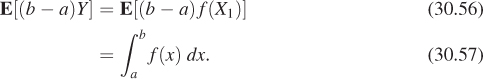
It seems intuitively obvious that the expected value here is still the integral of f on [a, b]. Let’s verify that. In mathematical terms, we have two random variables, X1 and X2, each with a uniform distribution on [a, b]. We then compute ![]() . What is E[(b – a)Y]? Using the linearity of expectation, we see that
. What is E[(b – a)Y]? Using the linearity of expectation, we see that
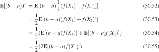
The last equality follows because X1 and X2 have the same distribution. Thus it follows that
What about the variance?
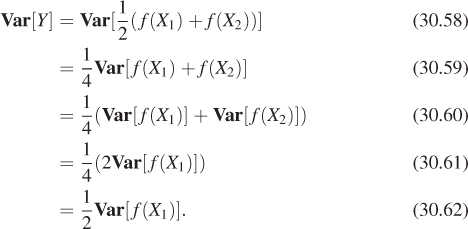
When we averaged two samples, the expectation remained the same, but the variance went down by a factor of two. (The standard deviation went down by a factor of ![]() ). If we define Yn by
). If we define Yn by
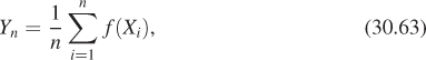
where the Xis are all uniformly distributed on [a, b], and are all independent, then the expected value of (b – a)Yn, for n = 1, 2, ..., is ![]() , while the variance of Yn is
, while the variance of Yn is ![]() .
.
This sequence of random variables has the property that as n goes to infinity, the variance goes to zero. That (together with the fact that ![]() for every n) makes it a useful tool in estimating the integral: We know that if we take enough samples, we’ll get closer and closer to the correct value.
for every n) makes it a useful tool in estimating the integral: We know that if we take enough samples, we’ll get closer and closer to the correct value.
To bring these notions back to graphics, when we recursively ray-trace, we find a ray-surface intersection, and then, if the surface is glossy, recursively trace a few more rays from that intersection point (using the BRDF to guide our random choice of recursive rays). At the next pixel in the image, we may hit a nearby point on the glossy surface, and trace a different few recursive rays, again chosen randomly. We are using those few recursive ray samples to estimate the total light arriving at the glossy surface (i.e., to estimate an integral). Even if the light arriving at the two nearby points of the surface is nearly identical, our estimates of it may not be identical. This leads to the appearance of noise in the image. The fact that choosing more samples leads to reduced variance in the estimator means that if we increase the number of recursive rays sufficiently, the noise they cause in the image will be insignificant.
In general, we’ve got some quantity C (like the integral of f, above), that we’d like to evaluate, and some randomized algorithm that produces an estimate of C. (Or, on the mathematical side, we have a random variable whose expectation is [or is near] the desired value.) We call such a random variable an estimator for the quantity. The estimator is unbiased if its expected value is actually C. Generally, unbiased estimators are to be preferred over biased ones, in the absence of other factors.
Estimators, being random variables, also have variance. Small variance is generally preferred over large variance. Unfortunately, there tend to be tradeoffs: Bias and variance are at odds with each other.
When we have a sequence of estimators like Y1, Y2, ... above, we can ask not whether Yk is biased, but whether the bias in Yk decreases to zero as k gets large, as does the variance. If both of these happen, then the sequence of estimators is called consistent. Clearly, consistency is a desirable property in an estimator: It suggests that as you do more work, you can be confident that the results you’re getting are better and better, rather than getting closer and closer to a wrong answer!
These are informal descriptions of estimators, bias, and consistency; making these notions really precise requires mathematics beyond the scope of this book. See, for example, Feller [Fel68].
30.5. Importance Sampling and Integration
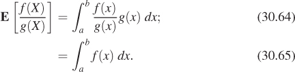
Let’s return for one more look at the problem of computing the integral of a function f on the interval [a, b], again as a proxy for computing the integral in the reflectance equation. In our previous efforts, we used uniformly distributed random variables to sample from the interval [a, b]. Now let’s see what happens when we use a random variable with some different distribution g. Since g will favor picking numbers in some parts of [a, b] over others, we can’t use the samples to directly estimate the integral as before. Instead, we have to compensate for the effect of g: We do the same computation as before, but include a division by g. The result is the importance-sampled single-sample estimate theorem.
Theorem: If f : [a, b] ![]() R is an integrable real-valued function, and X is a random variable on the interval [a, b], with distribution g, then
R is an integrable real-valued function, and X is a random variable on the interval [a, b], with distribution g, then ![]() is a random variable whose expected value is
is a random variable whose expected value is ![]() .
.
The proof is almost exactly the same as before:
Suppose that X is uniformly distributed on [a, b]. What’s the pdf g for the variable X? What does this importance-sampled single-sample estimate say about integrating f using X to produce a sample? Is it consistent with the single-sample estimate theorem? What happened to the extra factor of (b – a)?
Just as before, if we use n samples instead of one, the variance of the estimate decreases as ![]() .
.
The value of this nonuniform-sampling technique is that if you make the density function g be exactly proportional to f, then something quite interesting happens: Each sample of the random variable ![]() is the same (i.e., the random variable
is the same (i.e., the random variable ![]() is a constant). This means that the variance of the estimator is zero!
is a constant). This means that the variance of the estimator is zero!
Unfortunately, to make g exactly proportional to f (i.e., g = Cf for some C) and to make it a probability distribution, we need
In other words, the constant C is just the inverse of the integral we’re hoping to compute. To get the ideal benefit of this approach, we’d need to know the answer to the problem we’re trying to solve!
All is not lost, however. Suppose that the function g is larger where f gets larger, and smaller where f gets smaller, etc., albeit not in exact proportion. Then the variance of the weighted-sampling estimator is lower than that of the uniform-sampling approach. The use of such a function g is known as importance sampling, and g is sometimes called an importance function.
In practice in graphics, for a scene containing only reflection, we’re usually trying to estimate the integral that appears in the middle of the rendering equation,
for a fixed ωo and P. We know the reflectance function fr (it’s a property of the material at P), but we usually don’t have much idea a priori about how the factor L varies as a function of ωi. But in the absence of other information, the product Lfr is likely to be larger when fr is large and smaller when fr is small. We can therefore hope to reduce variance in our estimate by choosing samples in a way that’s proportional to fr, or better still, proportional to ωi ![]() fr(P, ωi, ωo) ωi · n(P), which we call the cosine weighted BRDF. This may not be possible, but it may be possible to choose them in a way that’s at least related to fr or the cosine weighted BRDF. This can help reduce variance substantially. In fact, it’s easy to see where this kind of importance sampling will help most.
fr(P, ωi, ωo) ωi · n(P), which we call the cosine weighted BRDF. This may not be possible, but it may be possible to choose them in a way that’s at least related to fr or the cosine weighted BRDF. This can help reduce variance substantially. In fact, it’s easy to see where this kind of importance sampling will help most.
• If the surface is mostly lit by a few point lights, then the variation in L will usually dominate the variation in fr in determining where the integrand is large or small.
• If the surface is mostly lit by diffusely reflected light coming from all different places, but is itself highly specular, then the shape of fr dominates in determining the size of the integrand, and importance sampling with respect to the cosine weighted BRDF is likely to reduce variance a lot.
Unfortunately, when we build a rendering system, we don’t necessarily know what kind of scenes we’ll be rendering. It would be nice to be able to combine the two strategies (use the cosine weighted BRDF as the importance function, or use some approximation of the arriving light field as the importance function) in a way that varies according to the particular situation. A technique called multiple importance sampling (see Section 31.18.4) allows us to do just that.
30.6. Mixed Probabilities
We’ve discussed discrete and continuum probabilities, but there’s a third kind, which we’ll call mixed probabilities, that comes up in rendering. They arise exactly from the impulses in bidirectional scattering distribution functions (BSDFs), or the impulses caused by point lights. These are probabilities that are defined on a continuum, like the interval [0, 1], but are not defined strictly by a density. Consider the following program, for example:
1 if uniform(0, 1) > 0.6 :
2 return 0.3
3 else :
4 return uniform(0, 1)
Sixty percent of the time this program returns the value 0.3; the other 40% of the time it returns a value uniformly distributed on [0, 1]. The return value is a random variable that has a probability mass of 0.6 at 0.3, and a pdf given by d(x) = 0.4 at all other points. We’d like to be able to say that the pdf is given by
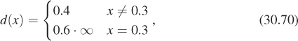
as shown schematically in Figure 30.10, but this makes no sense, literally. In the language of Chapter 18, we could instead say that the pdf was the sum of the constant function 0.4 and the delta function 0.6 · δ(x – 0.3). Or we can just say that it’s a random variable that has a probability mass at the point 0.3. In any case, a random variable with mixed probability is one for which there is a finite set of points in the domain at which the pdf is undefined, but for which there are associated positive probability masses rather than densities. The sum of the masses and the integral of the density over the remainder of the space must be 1.0.
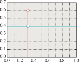
Figure 30.10: A mixed probability. The red stem (vertical line) indicates a probability mass. The blue graph (horizontal line) indicates a density.
The only critical feature of a random variable with a mixed probability is that when we want to integrate it via importance sampling, it’s important that we sample the locations of the probability masses with a nonzero probability. Since there are only finitely many probability masses, a good solution is the following.
1. Let x1, ..., xn be the locations of the probability masses.
2. Let M = Σimi ≤ 1 be the sum of the probability masses.
3. Let u = uniform(0, 1); if u ≤ M, return xi with probability mi/M.
4. Otherwise, return some value x using uniform or other sampling methods applicable to nonmixed probabilities.
In the example above, our approach would return x = 0.3 60% of the time, and return other values in the unit interval uniformly at random 40% of the time.
It’s not actually essential that the probability of picking xi be proportional to mi/M, but it’s an easy choice that makes the remaining computations in importance-weighted integration, for instance, much easier. We’ll see this applied in Chapter 32.
30.7. Discussion and Further Reading
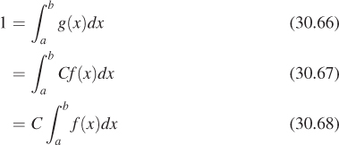
The key result of this chapter is the importance-sampled single-sample estimate theorem, with which we can estimate the integral of a function f over a region R by ![]() , where X is a random variable on the region R with distribution g. It lies at the heart of both ray-tracing and path-tracing algorithms. But also important are the notions of consistency and bias.
, where X is a random variable on the region R with distribution g. It lies at the heart of both ray-tracing and path-tracing algorithms. But also important are the notions of consistency and bias.
The use of Monte Carlo methods for integration is described, fairly densely, in Spanier and Gelbard’s classic book [SG69], where it’s applied to the study of neutron transport rather than photon transport.
30.8. Exercises
The first four exercises are designed to reinforce your understanding of Monte Carlo integration both without and with importance sampling.
Exercise 30.1: A friend picks three positive numbers A, B, and C and then draws the function graph shown in Figure 30.11. You don’t know the values A, B, and C. You get to ask your friend one question of the form “What is the value of f (s)?” for some particular s. Given these constraints, you are to estimate the integral of f over [0, 3]. Your approach is to flip a three-sided coin that lands on side i = 1, 2, or 3. You ask your friend, “What’s ![]() ?” You multiply his answer by three and use this as an estimate of the integral. The value produced is evidently a random variable, X.
?” You multiply his answer by three and use this as an estimate of the integral. The value produced is evidently a random variable, X.
(a) What’s the expected value μ = E[X]?
(b) What’s the variance of X? Express your answer in terms of A, B, C, and μ.
(c) Under what conditions on A, B, and C is the variance zero? Under what conditions is it large compared to μ?
Exercise 30.2: Continuing the preceding problem, suppose that instead of having a three-sided coin, you have a slightly broken random number generator, xrand, which returns a random number between 0 and 3. Seventy percent of the time it’s in [0, 1], uniformly distributed; 20% of the time it’s in [1, 2], uniformly distributed; and 10% of the time it’s in [2, 3], uniformly distributed. You’re given a single sample t generated by xrand, and you ask your friend to tell you y = f(t).
(a) Show how to use the value y to estimate the integral as before. Hint: Use importance sampling.
(b) Compute the variance of your estimate.
(c) When, qualitatively, would you expect the variance to be larger than that of the preceding problem’s estimator? When would you expect it to be lower?
(d) Write a short program to confirm that the expected value and variance really are what you predicted.
Exercise 30.3: Now imagine that instead of a function with three values, you had a function that took on infinitely many, such as ![]() .
.
(a) Compute the integral of h over [1, 3] using calculus.
(b) Estimate the integral of h over [1, 3] by writing a small program that picks a random number x uniformly in the interval, evaluates h there, and multiplies by 3 – 1. Run the program 100 times and average the results, and compare with your answer to part (a).
Exercise 30.4: In Equation 30.29, we showed that the pdf pW for the random variable W satisfied ![]() for every a and b in the interval [0, 1].
for every a and b in the interval [0, 1].
(a) Write ![]() , and compute f′(b) in terms of pW using the Fundamental Theorem of Calculus.
, and compute f′(b) in terms of pW using the Fundamental Theorem of Calculus.
(b) Since f(b) = b2 – a2 as well, compute f′ (b) in a different way.
(c) Conclude that pW(r) = 2r for any r ε [0, 1].
Exercise 30.5: Importance sampling.
(a) Compute the integral of f(x) = x2 on the interval [0, 1] using calculus.
(b) Use stochastic integration (with uniformly distributed samples) to estimate the integral, using n = 10, 100, 1,000, and 10,000 samples.
(c) Plot the error as a function of the number of samples. Repeat three times.
(d) Do the same computation, but for f (x) = cos2(x)e–20x.
(e) Use nonuniformly distributed samples to estimate the integral again, where the probability density of generating the sample x is proportional to s(x) = e–20x. To do this, you’ll need to determine the constant of proportionality; fortunately, that’s easy because s is easy to integrate on the interval [0, 1]. You’ll also need to generate samples with density proportional to s; the simplest approach is to generate a uniform sample, u ε [0, 1], and compute x = – ln(u)/20. If x is larger than 1, ignore it and repeat the process.
(f) Does this produce better estimates of the integral? Try to give an intuitive explanation of your conclusion.
Exercise 30.6: Consistency and bias. Consider a random variable X ~ U(0, 1). We saw in the chapter that we can estimate its mean by averaging n samples; this estimator will be unbiased. But consider the estimator
where the Xi are iid ~ U(0, 1).
(a) Show that each Yn is a biased estimator of the mean ![]() .
.
(b) Show that the sequence Y1, Y2, ... is a consistent estimator of the mean.
(c) Construct a sequence Zn of unbiased estimators that are not consistent. (Hint: Consistency requires two things.)
Exercise 30.7: Rejection sampling. In many cases where sampling from a distribution directly is difficult, rejection sampling is a last-resort solution that’s guaranteed to work, albeit very slowly in some cases. Figure 30.12 shows the idea: Drawing a box around the graph of a density function d, we select points uniformly randomly in the box. The x-values of these points are treated as samples, except that (x, y) is rejected (i.e., not used) if y > d(x). In areas where d(x) is large, a sample (x, y) is likely to be accepted; where d(x) is small, it’s likely to be rejected. When a sample’s rejected, we continue to generate new samples until we find an acceptable one.
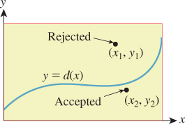
Figure 30.12: We draw a box around the graph of our probability density function d, and choose a point (x, y) uniformly randomly in the box. If (x, y) lies under the graph, we return x; if not, we try again.
(a) Write a program that uses rejection sampling to generate 10,000 samples from the distribution d(x) = x on the interval [0, 2] and plot your results in the form of a histogram.
(b) What fraction of your attempts at generating samples were rejected?
(c) Repeat with the distribution ![]() to see how badly rejection sampling can work.
to see how badly rejection sampling can work.
(d) Use the idea of rejection sampling (pick samples from a too-large space, and then select only the good ones) to generate points uniformly in the unit disk, and plot your results.
(e) Use the same idea to sample from the unit ball in 3-space, and the unit ball in 10-space. How well (in terms of rejection) does the last of these work?
(f) Points in the unit ball in any dimension are uniformly distributed in direction (with the exception of the origin). Use this to take your points-in-a-ball sampler and make a points-on-a-sphere sampler, being sure to reject the special case of the origin. Experimentally compare its efficiency to that of the hemisphere sampler we described. (Depending on your computer’s architecture, the comparison could go either way.)
(g) When you want to rejection-sample the function x ![]() 1+x on the interval [0, 1], you draw a box [0, 1] × [a, b] for some values a and b. What are the constraints on possible values for a and b? What happens if you make b quite large?
1+x on the interval [0, 1], you draw a box [0, 1] × [a, b] for some values a and b. What are the constraints on possible values for a and b? What happens if you make b quite large?
Exercise 30.8: Suppose that X is a random variable on [0, 1] with density e : [0, 1] ![]() R, and that f : [a, b]
R, and that f : [a, b] ![]() [0, 1] is a bijective increasing differentiable function.
[0, 1] is a bijective increasing differentiable function.
(a) Show that t ![]() e(f (t))f′(t) is a probability density on [a, b].
e(f (t))f′(t) is a probability density on [a, b].
(b) Suppose that Y is a random variable distributed according to t ![]() e(f(t))f′(t). Suppose that t0 ε [a, b] and x0 = f(t0). How are Pr{t0 – ≤ Y ≤ t0 + ε} and Pr{x0 – ≤ X ≤x0 + ε} related, for small values of ε? This whole problem is merely an exercise in chasing definitions—there should be no difficult mathematics involved.
e(f(t))f′(t). Suppose that t0 ε [a, b] and x0 = f(t0). How are Pr{t0 – ≤ Y ≤ t0 + ε} and Pr{x0 – ≤ X ≤x0 + ε} related, for small values of ε? This whole problem is merely an exercise in chasing definitions—there should be no difficult mathematics involved.
Exercise 30.9: Use the linearity of expectation repeatedly to show that Var[X] = E[X2] – E[X]2.
Exercise 30.10: Densities. Suppose that ([0, 1], p) is a probability space, that is, p is a probability density. We observed that p may take on values larger than 1. In this problem, you’ll show that this cannot happen too often. Show that if p(x) ≥ M on the interval a ≤ x ≤ b ![]() [0, 1], then b – a ≤
[0, 1], then b – a ≤ ![]() . Hint: Write out the probability of the event [a, b] as an integral, and then use the assumption about p to give a lower-bound estimate of this integral.
. Hint: Write out the probability of the event [a, b] as an integral, and then use the assumption about p to give a lower-bound estimate of this integral.