
Chapter 19. Enlarging and Shrinking Images
19.1. Introduction
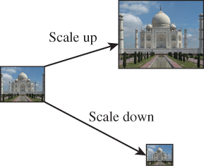
In Chapters 17 and 18 you learned how images are used to store regular arrays of data, typically representing samples of some continuous function like “the light energy falling on this region of a synthetic camera’s image plane.” You also learned a lot of theoretical information about how you can understand such sampled representations of functions by examining their Fourier transforms. In this chapter, we apply this knowledge to the problems of adjusting image sizes (scaling images up and down, as shown in Figure 19.1, which are synonyms for “enlarging” and “shrinking”), and performing various operations such as edge detection.
We assume that the values stored in an image array form a signal that is real-valued, not discrete; nothing we say here applies to an object-ID image, for example.
Just as we did in Chapter 18, in this chapter we study primarily grayscale images. Scaling up or down a grayscale image entails all the main ideas without the complications of three color channels. Furthermore, we continue to study the effects of transformations on a single row of image pixels, because the extension to two dimensions really has no important properties beyond those of one dimension, but the notation is substantially more complex. We do, however, return to two dimensions when providing code for scaling up and down, and when we analyze the efficiency of computing convolutions.
In this chapter, we use the following ideas from Chapter 18.
• Sampling and convolution operations on a signal can be profitably viewed in both the value and the frequency domains.
• The convolution-multiplication theorem. Convolution in the value domain corresponds to multiplication in the frequency domain, and vice versa.
• The transform of the unit-width box-function b is the unit-spacing sinc function, ![]() , while the transform of sinc is the box b.
, while the transform of sinc is the box b.
• The scaling property. If g(x) = f (ax), then
• Band limiting and reconstruction. If
– f is a function in L2(R), and
– ![]() (f)(ω) = 0 for |ω| ≥
(f)(ω) = 0 for |ω| ≥ ![]() , and
, and
– yi is the sample of f at i for i ![]() Z
Z
then f can be reconstructed from the yi’s by convolution with sinc, that is,
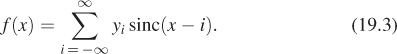
Furthermore, if f is not band-limited at ![]() , then sampling of f will produce aliases, in the sense that there is a band-limited function g whose samples are the same as those of f, and reconstruction using Equation 19.3 will produce g rather than f.
, then sampling of f will produce aliases, in the sense that there is a band-limited function g whose samples are the same as those of f, and reconstruction using Equation 19.3 will produce g rather than f.
• A sequence of L2 functions that approach a comb with unit tooth-spacing have Fourier transforms that approach a comb with unit tooth-spacing. Rather than talking about sequences that approach a comb, we’ll use the symbol Ψ as if there really were such a thing as a “comb function,” and you’ll understand that in any such use, there’s an implicit argument about limits being suppressed.
19.2. Enlarging an Image
In this and the next section, we’ll consider the problem of enlarging, or scaling up, and shrinking, or scaling down, an image. You might think that such operations would be straightforward, at least in some cases. If we have a 300×300 image, for example, and want a 150 × 150 version, it seems as if simply throwing away alternate rows and alternate columns would provide the desired result. Exercise 19.7 shows that this simple solution leads to very bad results, so we’ll need a different approach. Fortunately, the different approach we describe will solve the problem of scaling up and down not only by small integer factors, but by any factor at all. The scaling-up operation, which we address in this section, is relatively easy. The scaling-down operation, discussed in the next section, has additional subtleties.
We’ll work in one dimension as usual, so we’ll start with a 300-sample discrete signal (which we’ll call the source) that we want to turn into a 400-sample discrete signal (which we’ll call the target). We’ll assume that the 300-sample image was generated by sampling a function S ![]() L2(R) at 300 consecutive integer points.
L2(R) at 300 consecutive integer points.
We’ll also assume that the signal S : R ![]() R was strictly band-limited at ω0 =
R was strictly band-limited at ω0 = ![]() so that there was no aliasing when the samples were taken.
so that there was no aliasing when the samples were taken.
To resample S at 400 points, we’re going to imagine three idealized but impractical steps, which we’ll later refine to a practical algorithm.
1. Reconstruct S from the 300 samples in the image.
2. Stretch S along the x-axis by a factor of ![]() .
.
3. Resample S at the 400 sample points i = 0, ... 399.
When we reconstruct S in step 1, it’s band-limited at ω0 = ![]() . When we take 400 samples, if we want to avoid aliasing the signal must again be band-limited at
. When we take 400 samples, if we want to avoid aliasing the signal must again be band-limited at ![]() . Fortunately, when we stretch the signal S on the x-axis, the Fourier transform compresses along the ω-axis; the resultant signal is therefore still band-limited at
. Fortunately, when we stretch the signal S on the x-axis, the Fourier transform compresses along the ω-axis; the resultant signal is therefore still band-limited at ![]() . You can see, however, that when we want to shrink an image there will be additional challenges. Figure 19.2 shows this schematically.
. You can see, however, that when we want to shrink an image there will be additional challenges. Figure 19.2 shows this schematically.
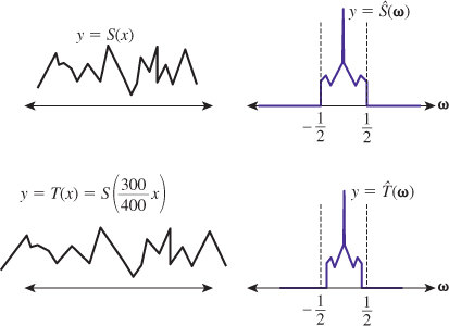
Figure 19.2: When the band-limited function S at left is stretched along the x-axis to form T, the transform of S at right is compressed, resulting in a more tightly band-limited transform.
There is a difficulty with the idea of reconstructing a signal from its samples at integer points. To do so, we need to know the value at every integer point, not just 300 of them. For now, we’re going to hide this problem by treating the source image outside the range 0 to 299 as being zero. We’ll return to this assumption in Section 19.4.
By the way, for a function f on Z or R, the support of f is the set of all places where it’s nonzero, that is,
If this set is contained in some finite interval, we say f has finite support; on the other hand, if the support is not contained in any finite interval, then f has infinite support. Thus, the box function has finite support, while sinc has infinite support. We’ve just chosen to treat our image samples as a function with finite support. With this assumption, we can recover the original signal S as shown in Listing 19.1. Note that rather than reconstructing the entire original signal, which would require an infinite amount of work, we’ve merely given ourselves the ability to evaluate this reconstructed signal at any particular point, thus converting the abstract first step into something practical.
Listing 19.1: Evaluating the original signal by convolving source image samples with sinc.
1 // Reconstruct a value for the signal S from 300 samples in the
2 // image called "source".
3 double S(x, source) {
4 double y = 0.0;
5 for (int i = 0; i < 300; i++) {
6 y += source[i] * sinc(x - i);
7 }
8 return y;
9 }
Notice that the sum is finite because we’ve assumed that source[i] is 0 except for i = 0, ..., 299. In general, the sum would have to be infinite, or, in practice, a sum over a very wide interval.
Now that we’ve reconstructed the original band-limited function, S, we need to scale it up to produce a new function T. If we think of each sample of S as representing the value of S at the middle of a unit interval, then the 300 samples we have for S, at locations 0, ..., 299, represent S on the interval [–0.5, 299.5]. We want to stretch this interval to [–0.5, 399.5].
To do so, we write
Once again, rather than building the signal T, we’ve merely provided a practical way to evaluate it at any point where we need it.
We must now sample T at integer locations. Since T is band-limited, it must be continuous, so sampling at x amounts to evaluation at x.
Clearly the numbers 300 and 400 can be generally replaced by numbers N and K where K > N, and every step of the process remains unchanged. The resultant code is shown in Listing 19.2.
Listing 19.2: Scaling up a one-dimensional source image.
1 // Scale the N-pixel source image up to a K-pixel target image.
2 void scaleup(source, target, N, K)
3 {
4 assert(K >= N);
5 for (j = 0; j < K; j++) {
6 target[j] = S((N/K) * (j + 0.5) - 0.5, source, N );
7 }
8 }
9
10 double S(x, source, N) {
11 double y = 0.0;
12 for (int i = 0; i < N; i++) {
13 y += source[i] * sinc(x - i);
14 }
15 return y;
16 }
To scale up a source image in two dimensions, we simply scale each row first, then scale each column (see Figure 19.3).
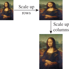
Figure 19.3: Scaling up rows and then columns to enlarge an image (Original image from http://en.wikipedia.org/wiki/File:Mona_Lisa,_by_Leonardo_da_Vinci,_from_C2RMF_retouched.jpg.)
Convince yourself that scaling rows-then-columns results in the same image as scaling columns-then-rows.
19.3. Scaling Down an Image
We now turn to the more complicated problem of scaling down an image I, that is, making it smaller. We’ll assume that the source image has N pixels and the target image has only K < N pixels.
Once again we can reconstruct from integer samples by convolving with sinc to get the original signal S. But in the next step, when we build
the resultant function is no longer band-limited at ![]() ; instead, it’s band-limited at
; instead, it’s band-limited at ![]() . Before we could safely sample T, we would have to band-limit it to frequency
. Before we could safely sample T, we would have to band-limit it to frequency ![]() by convolving with sinc.
by convolving with sinc.
Let’s look at the process in the frequency domain, as shown schematically in Figure 19.4. In reconstructing S, we convolved with sinc, that is, we multiplied by a width-one box in the frequency domain. When we squashed S to produce T, we stretched the Fourier transform of S correspondingly, and then needed to once again multiply by a unit-width box.
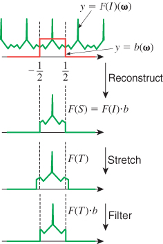
What if we instead multiplied by a box of width K/N before stretching, as shown in Figure 19.5? Then when we stretch the result by N/K, we’ll already be band-limited at ω0 = ![]() . So, in the frequency domain, the sequence of operations is as follows.
. So, in the frequency domain, the sequence of operations is as follows.
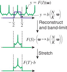
1. Multiply by ω ![]() b(ω) to reconstruct.
b(ω) to reconstruct.
2. Multiply by ω ![]() b((N/K)ω) to band-limit to
b((N/K)ω) to band-limit to ![]() .
.
3. Stretch by a factor of N/K; the result is band-limited at ![]() .
.
4. Convolve with Ψ as a result of sampling at integer points.
Notice that the first two steps can be combined: Multiplying by a wide box and then a narrow box gives the same result as multiplying by just the narrow box! This means that instead of reconstructing and then band-limiting, we can reconstruct and band-limit in a single step, by using a wider sinc-like function in the reconstruction process. Instead of x ![]() sinc(x), we need to use
sinc(x), we need to use ![]() . After that, all the remaining steps are the same. The program is shown in Listing 19.3.
. After that, all the remaining steps are the same. The program is shown in Listing 19.3.
Listing 19.3: Scaling down a one-dimensional source image.
1 void scaledown(source, target, N, K)
2 {
3 assert(K <= N);
4 for (j = 0; j < K; j++) {
5 target[j] = SL((N/K)* (j + 0.5) - 0.5, source, N, K);
6 }
7 }
8
9 // computed a sample of S, reconstructed and bandlimited at ![]() .
.
10 double SL(x, source, N, K) {
11 double y = 0.0;
12 for (int i = 0; i < N; i++) {
13 y += source[i] * (K/N) * sinc((K/N) * (x - i));
14 }
15 return y;
16 }
19.4. Making the Algorithms Practical
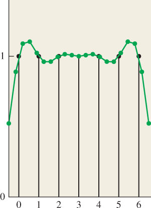
These are almost practical algorithms for image scaling. They both, however, rely on the assumption that we can use zeroes for the samples outside the source image; the result is that near the edges of the reconstructed source function, there are reduced values. For instance, suppose we start with a 7-pixel image, where every pixel has the value 1, and we scale up to a 20-pixel image. Figure 19.6 shows the seven pixels in a black stem plot, with the 20 pixels drawn in a connected green path on top of them. For pixels near the edges, ringing gives values that are greater than 1, and very near the edges the values are close to 0.
There are five solutions, shown schematically in Figure 19.7, none of them perfect.
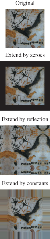
1. Extend by zeroes, which we’ve used so far.
2. Extend by reflection.
3. Extend by constants.
4. Limit the reconstruction filter to finite support, and use one of the approaches above.
5. Adjust the filter near the edges to ignore missing values.
We already discussed the problem with option 1: If we try to reconstruct a constant image, we get ringing artifacts at the edges as the band-limited function tries to drop to zero as quickly as possible. The benefit, however, is clear: We can limit our infinite summation to a finite one.
Option 2, in which we “hallucinate” some values for pixels outside the source image, fails to produce an L2 function, for if we reflect the source image each time we reach an edge, we create a tiling of the plane by copies of the source image; the L2 norm of this is infinitely many times the L2 norm of the source image, that is, ∞.
Option 3 means that as you examine one row of the image and run off the right-hand side of the image, you simply reuse the last pixel in the row as the value of all subsequent pixels, and you do the corresponding thing for the left, top, and bottom edges, and even the corners. This too leads to a signal that’s not in L2.
Although options 2 and 3 lead to signals that are not in L2, one solution is to say that reconstruction with the sinc is unrealistic: How can a sample at some point that’s miles away affect the value at a point within the image? Indeed, since the effect falls off as the inverse distance, that miles-away point will tend to have very little impact on the reconstruction. We can replace the sinc filter with some new filter g that looks like sinc but has finite support, and hope that its Fourier transform looks like the box function b. Unfortunately, it’s impossible for a function f ![]() L2(R) to have finite support and have
L2(R) to have finite support and have ![]() also have finite support [DM85]. But we can find finitely supported filters whose transforms are nearly zero outside a small interval, as we’ll discuss presently. If we agree to replace sinc by such a filter, then the whole question of whether the extension of the source image is L2 disappears: We can simply extend the source image by an amount R that’s greater than the support of the filter, and then fill in with zeroes beyond there. This is option 4, listed above.
also have finite support [DM85]. But we can find finitely supported filters whose transforms are nearly zero outside a small interval, as we’ll discuss presently. If we agree to replace sinc by such a filter, then the whole question of whether the extension of the source image is L2 disappears: We can simply extend the source image by an amount R that’s greater than the support of the filter, and then fill in with zeroes beyond there. This is option 4, listed above.
Finally, option 5 presents one last approach that’s somewhat unprincipled, but works well in practice. When we compute the value for a pixel with a summation of the form
we’re computing a weighted sum of source pixels. In this particular case, the weights come from the sinc function, but more generally we’re computing something of the form
where w is a list of weights. If these weights don’t sum to one, then filtering a constant image results in an image whose values are different from that constant. An example, based on filtering in the horizontal direction with a truncated sinc, is shown in Figure 19.8. The constant signal is shown in blue; it was sampled at integer points and reconstructed with x ![]() 1.4sinc(1.4x), truncated for |x| > 3.5. The resultant function was sampled far more finely and plotted in green, showing substantial ripple.
1.4sinc(1.4x), truncated for |x| > 3.5. The resultant function was sampled far more finely and plotted in green, showing substantial ripple.
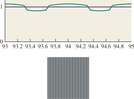
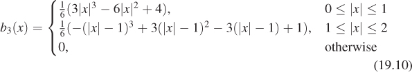
Figure 19.8: Top: Filtering a constant 1D signal with a truncated sinc leads to ripple. Bottom: A gray image, filtered and resampled with the same truncated sinc in the horizontal direction, ends up striped.
Typically, for things like a truncated sinc, the sum W of the weights is very close to one at each pixel. The sum may vary from one pixel to the next, however, resulting in a ripple when we try to reconstruct a constant image, as the figure shows. We can fix this problem somewhat by dividing by the sum of the weights at each pixel, which removes the ripple. In effect, we’ve altered the filter so that its Fourier transform is zero at all multiples of the sampling frequency. We’ve done so at the cost of modifying the filter, however, so its Fourier transform is no longer what we expected. As long as the ripple is small, though, the alteration to the function is small, and hence the alteration to the transform is small as well.
The useful characteristic of this unrippling operation is that it suggests a way to deal with the missing data at the edges of images as well: We compute the sum
but simply ignore all terms where source(i) is outside the image. We sum up the weights as usual, but only for the terms we included, and then divide by this sum. In the interior of the image, every pixel we need is available and we’re just unrippling. At the edges, we end up estimating the pixel values near the edge based only on the image pixels near the edge, and not on some hallucinated values on the other side of the edge. This method works surprisingly well in practice.
19.5. Finite-Support Approximations
We’ve said that the ideal reconstruction filter is sinc, but that it’s often necessary to compromise in practice and use a finite-support filter. We’ve already seen the box and tent filters, and that the tent is the convolution b * b of the box with itself. We can further convolve to get smoother and smoother filters as discussed extensively in Chapter 22, which is about the construction of piecewise-smooth curves. The convolution of the tent with itself (or b * b * b * b), known as the cubic B-spline filter and plotted in Figure 19.9, is shown in Chapter 22 to be
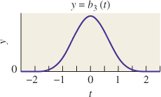
There is a slight difference from the function in Chapter 22, however: This chapter’s version of b3 has support [–2, 2], while in Chapter 22 the support is [0, 4].
Notice that b3(0) = ![]() , while b3(±1) =
, while b3(±1) = ![]() . This means that when we reconstruct an image using b3, the reconstructed value at the image points is not the original image value, but a blend between it and its two neighbors.
. This means that when we reconstruct an image using b3, the reconstructed value at the image points is not the original image value, but a blend between it and its two neighbors.
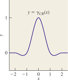
An alternative is the Catmull-Rom spline (see Chapter 22 for details), γCR, which is zero at every integer except γCR(0) = 1, as shown in Figure 19.10. This means that reconstructing with this filter leaves the image points unchanged, and merely interpolates values between them. On the other hand, the CatmullRom spline takes on negative values, which means that interpolating with it may produce negative results, which is a problem: We can’t have “blacker than black” values. The formula for the Catmull-Rom spline is

A ![]() blend of the Catmull-Rom curve and the B-spline curve was recommended by Mitchell and Netravali [MN88] as the best all-around cubic to use for image reconstruction and resampling. That filter (shown in Figure 19.11) is given by
blend of the Catmull-Rom curve and the B-spline curve was recommended by Mitchell and Netravali [MN88] as the best all-around cubic to use for image reconstruction and resampling. That filter (shown in Figure 19.11) is given by
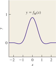
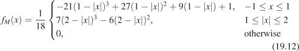
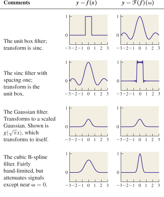
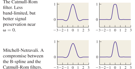
Table 19.1 shows several filters and their Fourier transforms.
19.5.1. Practical Band Limiting
The function sinc is band-limited at ω0 = ![]() . The cubic B-spline filter b3 is not, and it passes frequencies much larger than
. The cubic B-spline filter b3 is not, and it passes frequencies much larger than ![]() , albeit attenuated. As we showed in Chapter 18, the consequence of this is aliasing. A signal at frequency 0.5 + a appears as an alias at frequency 0.5 – a. In particular, integer-spaced samples of a signal of frequency near 1 look like samples of a signal of frequency near 0. Indeed, any near-integer frequency aliases to a low frequency.
, albeit attenuated. As we showed in Chapter 18, the consequence of this is aliasing. A signal at frequency 0.5 + a appears as an alias at frequency 0.5 – a. In particular, integer-spaced samples of a signal of frequency near 1 look like samples of a signal of frequency near 0. Indeed, any near-integer frequency aliases to a low frequency.
If we use a filter like b3 to reconstruct a continuum signal from image data, the resultant signal will contain aliases, because the support of ![]() is not contained in H = (–
is not contained in H = (–![]() ]. Fortunately, outside H the Fourier transform falls off fairly rapidly; nonetheless, there is some aliasing.
]. Fortunately, outside H the Fourier transform falls off fairly rapidly; nonetheless, there is some aliasing.
We can address this with a compromise: We can stretch b3 along the x-axis so that the Fourier transform compresses along the ω-axis, pushing more of the support inside H and reducing aliasing. This has the unfortunate consequence that frequencies that we’d like to preserve, near ± ![]() , end up attenuated. The compromise involved is one of trading off blurriness (i.e., a lack of frequencies near |ω| =
, end up attenuated. The compromise involved is one of trading off blurriness (i.e., a lack of frequencies near |ω| = ![]() ) against low-frequency aliasing (i.e., frequencies near |ω| = 1). For frequencies in between these extremes, aliasing still occurs. But if a frequency just above
) against low-frequency aliasing (i.e., frequencies near |ω| = 1). For frequencies in between these extremes, aliasing still occurs. But if a frequency just above ![]() aliases to one just below
aliases to one just below ![]() , it’s often removed during image shrinking anyhow, and in practice turns out to not be as noticeable as an alias at a frequency near 0.
, it’s often removed during image shrinking anyhow, and in practice turns out to not be as noticeable as an alias at a frequency near 0.
19.6. Other Image Operations and Efficiency
In general, convolving an image with a discrete filter of small support can be an interesting proposition. We already saw how convolving with a 3 × 3 array of ones can blur an image (although to keep the mean intensity constant, you need to divide by nine).
In general, we can store a discrete filter in a k × k array a, and the image in an n × n array b; the result of the convolution will then be an (n + k) × (n + k) array c; the code is given in Listing 19.4.
Listing 19.4: Convolving using the “extend by zeroes” rule.
1 void discreteConvolve (float a[k][k], float b[n][n], float c[n+k-1][n+k-1])
2 initialize c to all zeroes
3 for each pixel (i,j) of a
4 for each pixel (p, q) of b
5 row = i + p;
6 col = j + q;
7 if (row < n + k - 1) && (col < n + k - 1))
8 c[row][col] += a[i][j] * b[p][q];
A much nicer blur than the one we saw with the box filter comes from convolving with a Gaussian filter, that is, samples of the function ![]() exp(-
exp(-![]() ), where σ is a constant that determines the amount of blurring: If σ is small, then the convolution will be very blurry; if it’s large, there will be almost no blurring. The value σ = 1 produces a bit less blurring than convolving with a 3 × 3 array of ones. You can also blur preferentially in one direction or another, using a filter defined by
), where σ is a constant that determines the amount of blurring: If σ is small, then the convolution will be very blurry; if it’s large, there will be almost no blurring. The value σ = 1 produces a bit less blurring than convolving with a 3 × 3 array of ones. You can also blur preferentially in one direction or another, using a filter defined by
where S is any symmetric 2 × 2 matrix. The axes of greatest and least blurring are the eigenvectors of S corresponding to the least and greatest eigenvalues, respectively. The amount of blur is inversely related to the magnitude of the eigenvalues.
If B is any blurring filter, and your image is I, then B* I is a blurred version of I; roughly speaking, convolution with B must remove most high frequencies from I, leaving the low-frequency ones. This means that if we compute I – rB* I for some small r > 0, we’ll be removing the blurred version and should leave behind a sharpened version. Unfortunately, this also darkens the image: If I initially contains all ones, then all entries of I – rB* I will be 1 – r. We can compensate by using
to sharpen the image. In the case where B is the 3 × 3 box 1 9
the result is
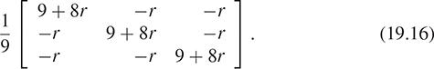
The results, using r = 0.6, are shown in Figure 19.12, where the blur and sharpening have been applied to a very low-resolution version of the Mona Lisa, magnified so that you can see individual pixels.
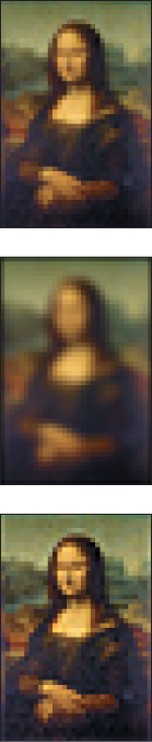
You can apply this idea to any blurring filter B to get an associated sharpening filter.
If we convolve an image I with the 1 × 2 filter [1 –1], it will turn any constant region of I into all zeroes. But if there’s a vertical edge (i.e., a bright pixel to the left of a dark pixel), the convolution will produce a large value. (If the bright pixel is to the right of the dark one, it will produce a large negative value.) Thus, this filter serves to detect (in the sense of producing nonzero output) vertical edges. A similar approach will detect horizontal edges. And using a wider filter, like [1 1 1 –1 –1 –1], will detect edges at a larger scale, while producing relatively little output for small-scale edges. By computing both the vertical and horizontal “edge-ness” for a pixel, you can even detect edges aligned in other directions. In fact, if we define
then [H(i, j) V(i, j)] is one version of the image gradient at pixel (i, j)—the direction, in index coordinates, in which you would move to get the largest increase in image value.
The images H and V are slightly “biased,” in the sense that H takes a pixel to the right and subtracts the current pixel to estimate the change in I as we move horizontally, but we could equally well have taken the current pixel minus the pixel to the left of it as an estimate. If we average these two computations, the current pixel falls out of the computation and we get a new filter, namely ![]() [–1 0 1]. This version has the advantage that the value it computes at pixel (i, j) more “fairly” represents the rate of change at (i, j), rather than a half-pixel away. Figure 19.13 shows the blurred low-resolution Mona Lisa, the result of [–1 0 1] -based edge detection along rows and along columns, and a representation of the gradient computed from these. (We’ve trimmed the edges where the gradient computation produces meaningless results.)
[–1 0 1]. This version has the advantage that the value it computes at pixel (i, j) more “fairly” represents the rate of change at (i, j), rather than a half-pixel away. Figure 19.13 shows the blurred low-resolution Mona Lisa, the result of [–1 0 1] -based edge detection along rows and along columns, and a representation of the gradient computed from these. (We’ve trimmed the edges where the gradient computation produces meaningless results.)
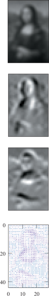
Figure 19.13: Mona Lisa, row-wise edge detection, column-wise edge detection, and a vector representation of the gradient.
For more complex operations like near-perfect reconstruction, or edge detection on a large scale, we need to use quite wide filters, and convolving an N × N image with a K × K filter (for K < N) takes about K2 operations for each of the N2 pixels, for a runtime of O(N2K2). If the K × K filter is separable—if it can be computed by first filtering each row and then filtering the columns of the result—then the runtime is much reduced. The row filtering, for instance, takes about K operations per pixel, for a total of N2K operations; the same is true for the columns, with the result that the entire process is O(N2K), saving a factor of K.
19.7. Discussion and Further Reading
It’s clear that aliasing—the fact that samples of a high-frequency signal can look just like those of a low-frequency signal—has an impact on what we see in graphics. Aliasing in line rendering causes the high-frequency part of the line edge to masquerade as large-scale “stair-steps” or jaggies in an image. Moiré patterns are another example. But one might reasonably ask, “Why, when the eye is presented with such samples, which could be from either a low- or a high-frequency signal, does the visual system tend to interpret it as a low one?” One possible answer is that the reconstruction filter used in the visual system is something like a tent filter—we simply blend nearby intensities together. If so, the preferred reconstruction of low frequencies rather than high frequencies is a consequence of the rapid falloff of the Fourier transform of the tent. Of course, this discussion presupposes that the visual system is doing some sort of linear processing with the signals it receives, which may not be the case. At any rate, it’s clear that without perfect reconstruction, even signals near the Nyquist rate can be reconstructed badly, so it may be best, when we produce an image, to be certain that it’s band-limited further than required by the pure theory. The precise tuning of filter choices remains something of a dark art.
Digital signal processing, like the edge detection, blurring, and sharpening mentioned in this chapter, is a rich field. Oppenheim and Schafer’s book [OS09] is a standard introduction. Many of the obvious techniques don’t work very well in practice. Our example of edge detection and gradient finding with the Mona Lisa was carefully applied to a blurred version of the image, because the unblurred version generated many edges and the gradients appeared random. Such tricks form an essential part of the tool set of anyone who works with image data.
19.8. Exercises
![]() Exercise 19.1: Suppose you’re building a ray tracer and you want to build a 100 × 100 grid on the image plane. The image plane has uv-coordinates on it, and the image rectangle ranges from –
Exercise 19.1: Suppose you’re building a ray tracer and you want to build a 100 × 100 grid on the image plane. The image plane has uv-coordinates on it, and the image rectangle ranges from –![]() to
to ![]() in u and v. Where should you place your samples? Consider the one-dimensional problem instead: We need 100 samples between u = –
in u and v. Where should you place your samples? Consider the one-dimensional problem instead: We need 100 samples between u = –![]() and u =
and u = ![]() . One choice is ui = –
. One choice is ui = –![]() + (i/99), i = 0, ..., 99. These points range from u0 = –
+ (i/99), i = 0, ..., 99. These points range from u0 = – ![]() to u99 =
to u99 = ![]() . The other natural choice is to space the points evenly so that they are separated by 1/100, that is, ui = –
. The other natural choice is to space the points evenly so that they are separated by 1/100, that is, ui = –![]() + (i/100) + (1/200).
+ (i/100) + (1/200).
(a) Suppose that instead of 100 points, you want N = 3 points. Plot the ui for each method.
(b) Do the same for N = 2 and N = 1.
(c) Imagine that instead of 100 points ranging from –![]() to
to ![]() , you wanted 200 points ranging from –1 to 1. You might expect the “middle” 100 points from this wider problem to correspond to your 100 points for the narrower problem. Which formula has that property?
, you wanted 200 points ranging from –1 to 1. You might expect the “middle” 100 points from this wider problem to correspond to your 100 points for the narrower problem. Which formula has that property?
Exercise 19.2: One favorite filter is the Gaussian, defined by g(x, y) = Ce–π(x2+y2). It has three important properties. First, it is its own Fourier transform. Second, it’s circularly symmetric: Its value on the circle of radius r around the origin is constant. Third, it’s a product of two one-dimensional filters. Do the algebra to show the second and third properties.
![]() Exercise 19.3: The cubic spline filter B can be converted into a circularly symmetric filter on the plane by saying
Exercise 19.3: The cubic spline filter B can be converted into a circularly symmetric filter on the plane by saying ![]() . Unfortunately, this circularly symmetric filter is not separable. The separable filter C(x, y) = B(x)B(y) built from B is not circularly symmetric. How different are they? Numerically estimate the integral of C(x, y) –
. Unfortunately, this circularly symmetric filter is not separable. The separable filter C(x, y) = B(x)B(y) built from B is not circularly symmetric. How different are they? Numerically estimate the integral of C(x, y) – ![]() (x, y) over the plane.
(x, y) over the plane.
Exercise 19.4: Apply the unrippling approach, with the missing-weights modification, on the cubic B-spline filter, applied to scaling up a signal by a factor of 10.
(a) Apply the technique to a ten-sample signal where every sample value is 1.
(b) Apply it to a ten-sample signal where sample i is cos(πki/20) for k = 1, 4, and 9. Comment on the results.
Exercise 19.5: Here’s an alternative approach to reconstructing a band-limited signal from its samples.
(a) Argue why the operation must be well defined (i.e., why there is exactly one signal in L2(R), band-limited at ω0 = ![]() , with any particular set of values on the integers).
, with any particular set of values on the integers).
(b) Argue that reconstruction must be linear, that is, if fi : R ![]() R is the reconstruction of the discrete signal si : Z
R is the reconstruction of the discrete signal si : Z ![]() R for i = 1, 2, then f1 + f2 is the reconstruction of the discrete signal s1 + s2.
R for i = 1, 2, then f1 + f2 is the reconstruction of the discrete signal s1 + s2.
(c) Argue that if for some k, s3(n) = s1(n + k) for every n ![]() Z, then the reconstruction f3 of s3 is just f3(x) = f1(x+k). We say that reconstruction is translation equivariant.
Z, then the reconstruction f3 of s3 is just f3(x) = f1(x+k). We say that reconstruction is translation equivariant.
(d) Explain why the reconstruction of the signal s with s(0) = 1, and s(n) = 0 for all other n, is just f(x) = sinc(x).
(e) From your answers to parts (a) through (d), conclude that reconstruction for any discrete signal comes from convolution with sinc.
Exercise 19.6: Suppose we band-limit f(x) = sinc(x) to ω0 = ![]() . Describe the resultant signal precisely.
. Describe the resultant signal precisely.
Exercise 19.7: We suggested that one bad way to downsample a 300 × 300 image to a 150 × 150 image was to simply take pixels from every second row and every second column. Suppose the source image is a checkerboard: Pixel (i, j) is white if i + j is even, and it’s black if it’s odd. At a distance, this image looks uniformly gray.
(a) Show that if we choose pixels from rows and columns with odd indices, the resultant subsampled image is all white.
(b) Show that if we use odd row indices, but even column indices, the resultant subsampled image is all black.