
Chapter 26. Light
26.1. Introduction
We now turn to a more formal discussion of light, expanding considerably on the simple ideas from Section 1.13.1. We start with the physical properties of light, one of which is that it has many characteristics of waves, including a frequency. Our eyes perceive lights of different frequencies as having different colors, but since color is a perceptual phenomenon rather than a physical one, we treat it separately in Chapter 28.
The second part of this chapter is about the measurement of light and the various physical units we use to describe light. Since almost all of these can be described as integrals of one basic quantity (radiance), we also briefly discuss a few special integrals that arise often in rendering. Finally, although it is not strictly a property of light, we introduce the measurement of the reflection of light by surfaces, and compute the light reflected from a surface in two simple situations.
26.2. The Physics of Light
We live in a world in which electromagnetic radiation is everywhere. We’re constantly bathed in both heat and light arriving from the sun, radio and television signals are present almost everywhere on Earth, etc. Light refers to a particular kind of electromagnetic radiation (of a frequency that can be detected by the human eye, or nearly so). Because of this relationship to the human eye, light has, over the years, been described not only in physical terms (like energy) but also in perceptual terms, things having to do with the way that the human visual system processes and perceives light. The most obvious of these is color, which we discuss in the next chapter in detail. We begin with the characteristics of the radiation at microscopic and macroscopic scales, and then move on to a discussion of how light is measured. The study of the measurement of radiation in general is called radiometry, and radiometric ideas are relatively easy to grasp, as is radiometry applied to light (i.e., electromagnetic radiation of the kind that the human eye can detect). There’s a second way of measuring light, called photometry, which is closely related to the human visual system; photometric measures of light tend to be summary measures, in that they measure things that can be computed from radiometric quantities by computing weighted sums. We’ll touch on these measurement topics later in this chapter and the next.
At a macroscopic level, light can be regarded as a kind of energy that flows uninterrupted through empty space along straight lines, but is absorbed into and/or reflected from surfaces that it meets. At a microscopic level, light turns out to be quantized—it comes in individual and indivisible packets called photons. At the same time, light is wavelike—it is a kind of electromagnetic radiation and is characterized in part by a frequency, f. The energy E of a photon and the frequency f are related by
where λ is the wavelength of the light in meters, c ≈ 2.996 × 10⁸ ms–1 is the speed of light, which is constant in a vacuum, and h ≈ 6.626 × 10⁻³⁴ kg m2 s–1 is Planck’s constant.
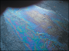
In graphics, we generally are interested in the macroscopic phenomena, and therefore we ignore the indivisibility of photons. But there are phenomena where the microscopic characteristics of light are important, particularly the wavelike characteristics. Since light is an electromagnetic phenomenon, it’s actually described by both electric and magnetic characteristics; the magnetic characteristics are determined by the electrical ones, so we’ll mostly ignore them. The electrical wavelike characteristics produce the phenomenon called polarization. Effects of the wavelike characteristics, including refraction and polarization, are actually important in some phenomena that we see in day-to-day life, such as the colors reflected by gemstones, the appearance of rainbows, the rainbow patterns seen on diffraction gratings, the colors seen in a thin layer of oil or gasoline on water (see Figure 26.1), the scattering of light by colloidal suspensions like milk, and the scattering of light through multilayered surfaces like human skin.
We begin with the microscopic view because of its importance in explaining certain color phenomena, for instance, and because we feel that those working with light on a day-to-day basis should know something about its physical properties. But this material can safely be skipped by those who are only interested in high-level phenomena and are willing to take for granted certain claims about radiation that we’ll make when discussing color.
We then continue with the macroscopic view, which can be easily understood by analogy with everyday phenomena.
26.3. The Microscopic View
In this section we’ll give a high-level overview of the nature and production of light; those interested in further details should begin with a good understanding of electricity and magnetism (we particularly recommend Purcell’s book [Pur11]).
Let’s start with a simple model of an atom consisting of a central nucleus surrounded by electrons, which we depict in Figure 26.2 as circling about the nucleus in orbit. Electrons in orbits farther from the nucleus have more energy than those close to the nucleus (just as it takes more energy to launch a high-orbit satellite around the Earth than a similarly sized low-orbit satellite). An electron can drop from a high-energy orbit to a lower-energy one; typically when this happens, a photon is emitted; its energy is the difference between the two energy levels. An atom can also absorb a photon of energy E by having some electron move into a new orbit whose energy is exactly E higher than that of its current orbit. Sometimes there is no pair of orbits whose difference is exactly E; in this case, the photon cannot be absorbed by the atom. Electrons can also change levels through other mechanisms, one of which is vibration, in which some of the energy of an electron in a substance is converted to or from vibration of the atoms of the substance.
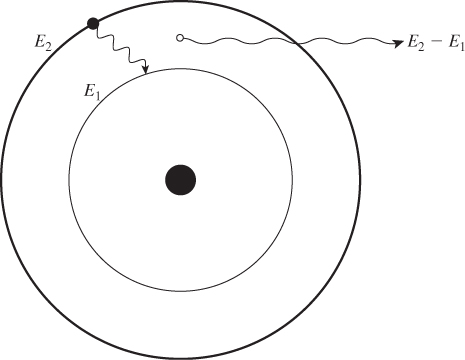
Figure 26.2: An atom has a nucleus around which electrons orbit in various orbital levels. Each orbital is associated with an energy level. An electron can “fall” from an orbital of higher energy, E2, to an orbital of lower energy, E1; when it does, a photon with energy E2 – E1 is emitted. The reverse can also happen: A photon with energy E2 – E1 can be absorbed by the atom, lifting the electron from the orbital of energy E1 to that of energy E2.
A typical phenomenon is that a photon is absorbed by an atom, raising the electron to a new energy level; the electron, some brief time later, then falls back down to the lower energy and a new photon is emitted. Sometimes the path to the lower energy level goes through an intermediate level: First some electron energy is converted to vibration, and then a photon-emitting energy jump takes place. The outgoing photon has a lower energy than did the incoming one; this phenomenon is called fluorescence. The most familiar examples are minerals which, when illuminated by ultraviolet light (sometimes called black light), emit visible light. There is a closely related phenomenon called phosphorescence, in which the transition from the intermediate state to the low-energy state is relatively unlikely, and therefore can take place over a long period of time. A phosphorescent material, illuminated by light, can continue to glow for some time after the illumination is removed. There’s one other form of interaction between a photon and an atom: Sometimes the photon kicks an electron to a higher energy state, from which it returns to the original state almost immediately; the result is that the photon continues on its original way, slightly delayed. The likelihood of such virtual transitions depends on the nature of the material, but the delay they induce has an important macroscopic effect: The speed of light through materials is slower than that in a vacuum, with the slowness being determined by how often such virtual transitions occur.
The simple model of discrete energy levels really applies only to an isolated atom. When multiple atoms are in proximity (as in solids), each individual energy level available to electrons gets “spread out” into a band of energies. Still, electrons can generally absorb or release energies only when the amount absorbed or released represents the difference of two energies in the bands.
In some materials—like metals—certain electrons are not attached to particular nuclei, but can instead move about the material, helping to make the material conductive. These electrons have a great many possible energy states, and therefore can absorb photons of many different wavelengths and then promptly emit them again. This generally makes conductive materials like metals reflective, while most transparent materials are insulators.
In other materials—like some forms of carbon—there are also unattached electrons, but they cannot move quite as freely. Such an electron can interact with atoms of the material, causing those atoms to move and vibrate while the electron loses energy. This motion of atoms is called heat. Thus, materials like soot tend to absorb photons, and rather than reemitting the photons, they convert them into heat. This is why soot looks black, and why dark clothes heat up on a sunny day. Note that light of all frequencies is convertible to heat. In particular, infrared light (light of wavelengths slightly longer than those we can see) is a kind of electromagnetic radiation, just like the light we see; it happens to be more readily convertible to heat than is visible light, but it’s still light.
In the exact reverse process, if we heat up soot, the atoms vibrate; this vibration in turn may “kick around” a loose electron, causing it to have excess energy, which it may lose by emitting a photon. Because of the many possible energy states for the loose electron, the emitted light can have many possible energies (wavelengths). Thus, materials that are good at absorbing energy and converting it to heat are also good at emitting energies of many different amounts when they are heated.
As materials are heated, they all become increasingly better at emitting electromagnetic radiation. Indeed, all bodies at all temperatures above absolute zero actually emit some radiation, but at the low temperatures we encounter in ordinary life, it’s not very much. We mostly see things because they are reflecting light rather than because they are emitting it themselves. The exceptions are things like the filaments in incandescent lightbulbs, hot metal being forged by a blacksmith, or the sun.
We can measure the energy radiated by an object heated to temperature T (see Figure 26.3). For each narrow range of wavelengths, we can measure the energy radiated in that range; plotting this function I(λ, T) against frequency λ gives a graph like that shown in Figure 26.4. At very low temperatures, such measurements are easily confounded with reflected energy. But if we imagine an ideal black body—one that can absorb and emit electrons as well as possible—in a room in which the only energy is in the form of heat, we get a plot like the one shown in the figure.
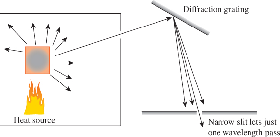
Figure 26.3: An object is heated to some temperature, and a narrow beam of the radiation it produces is focused on a diffraction grating, splitting it into energies of different wavelengths. By moving a plate with a slit in front of this diffracted energy, we can measure the energy radiated in a narrow range of wavelengths, [λ, λ + dλ].
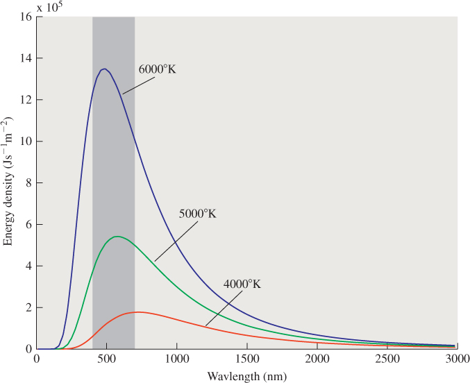
Figure 26.4: The radiation near wavelength λ from a black body heated to some temperature T, plotted as a function of λ, shown for several values of T. The shaded region indicates the wavelengths of visible light.
The dependence of I on T can be measured; the total power radiated depends on the fourth power of T:
power = σT4, where σ = 5.67 × 10⁻⁸ W m–2 K–4;
this is known as the Stefan-Boltzmann law. (The K in this expression denotes “degrees Kelvin.”)
On a warm day the temperature is about 300°K.
(a) What does the Stefan-Boltzmann law predict as the amount of energy radiated from your body? (You should assume that your surface area is about one square meter, and that you radiate as a black body.)
(b) When sitting at home on such a day, why do you not get very cold from this loss of heat?
The other notable feature in the graph is that the location of the peak radiation intensity moves to the left as the temperature increases. At about 900°K, there is enough radiation in the visible portion of the spectrum for the eye to detect it. As a first peek at color, we mention one thing: Radiation with a wavelength between about 400 nanometers and 700 nanometers is visible to the human eye; radiation at the 700-nanometer end of the spectrum looks red, and the appearance transitions through yellow, green, and cyan as the wavelength shortens (i.e., the energy increases); and radiation near the 400-nanometer end of the visible spectrum looks blue. Since at 900°K the radiated energy at the low-frequency (i.e., long-wavelength) end of the visible spectrum is larger than that at the high-frequency end, we see such an object glowing a dull red. As we heat it further, it becomes a great deal brighter because of the exponent of 4 in the Stefan-Boltzmann law. But higher frequencies begin to mix in, and we see a combination of red and green (i.e., an orange and then a yellow color) and eventually a combination of red, green, and blue, which we perceive as white. By the time an object is glowing white, it’s emitting energy at an amazing rate; at 5000°K, it’s radiating at about 35 megawatts per square meter. Clearly this radiation dominates whatever light the surface might reflect from the ordinary illumination in a room, for instance.
By the way, lamps used in filmmaking and photography are often described using temperatures; that’s shorthand for saying, “The spectrum of light emitted by this lamp is quite similar to that of black-body radiation of that temperature.” This can be useful in adjusting a scene to appear illuminated by ordinary incandescent lamps or by sunlight.
Max Planck developed an expression for the shape of the curve in the graph above, later supported by theoretical analysis based on quantum theory; he observed that
where h is Planck’s constant and k is Boltzmann’s constant (about 1.38 × 10– 23 JK–1). The precise values are not important to us, but the shape of the curve is. Because ex = 1+x + ..., the denominator of the second factor is, for large λ, roughly proportional to 1/λ, so I(λ, T) is proportional to λ–4; for small λ, the exponential dominates and the curve heads to zero. Note that I(λ, T)Δλ is the amount of energy at wavelengths between λ and λ +Δλ, for small values of Δλ; to find the total energy in some range of wavelengths, you have to integrate with respect to λ over that range. The corresponding expression, in terms of frequency, which is the more common descriptor used for light in physics, is
in which frequency appears to the third power, while wavelength appeared to the fifth power; this is because integration with respect to f involves a change of variables from λ to f, namely, λ = c/f, dλ = –c/f2df.
26.4. The Wave Nature of Light
As mentioned earlier, light is a kind of electromagnetic radiation. (Indeed, “light” is a general term for this, with “visible light” being the radiation that the human eye can detect. We’ll generally follow common usage and mean “visible light” when we speak of “light.”) Other kinds include X-rays, microwaves, etc. (see Figure 26.5). The wave nature of light is best used when trying to understand how light propagates; in fact, a good rule of thumb is that “[e]verything propagates like a wave and exchanges energy like a particle” [TM07]. To understand the propagation of light, we must discuss kinds of waves.
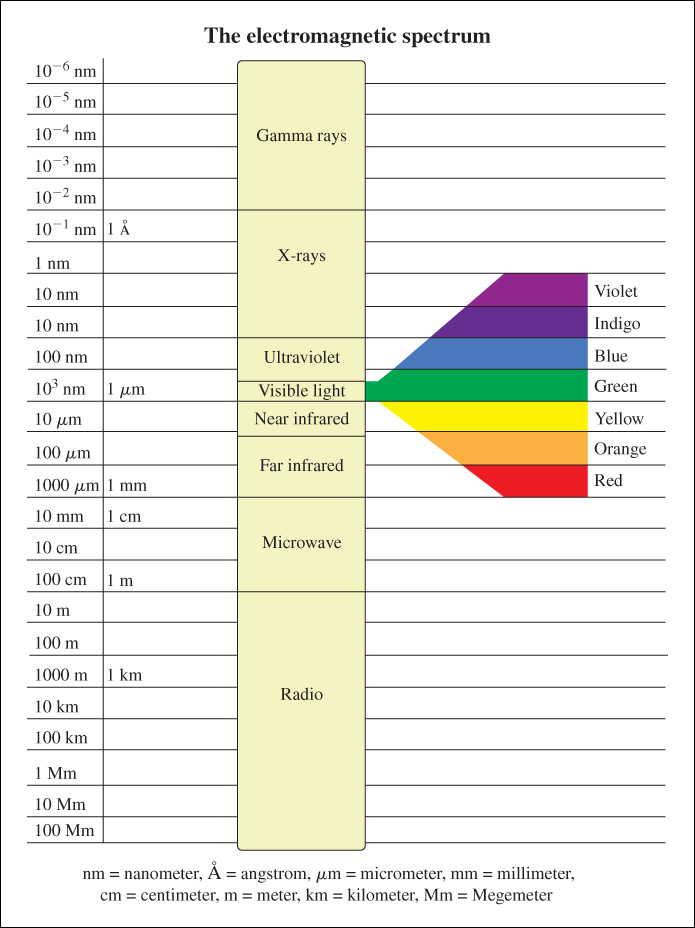
Figure 26.5: The electromagnetic spectrum includes many different phenomena; visible light occupies only a small portion of the spectrum.
Large and regular waves on the surface of the ocean are linear waves—each peak and trough consists of a long line that moves in a direction perpendicular to the axis of the line (see Figure 26.6). The wavelength is the perpendicular distance between adjacent peaks (or adjacent troughs). The wave velocity is the velocity with which the peak moves. This is not the velocity of any individual particle of water, which is easy to see by watching, for instance, a log floating on the surface: As waves pass, the log rises and falls, and may also move somewhat back and forth in the direction of the wave, but long after the peak of the wave has moved on, the log remains more or less where it started.

Figure 26.6: Ocean waves arriving at Panama City. The waves come in long lines, which have been slightly bent by the irregularities of the ocean floor as they approach the shore. (Courtesy of Nick Kocharhook.)
(a) A thin human hair has a diameter of 50 μm ≈ ![]() inch. Red light has a wavelength of about 700 nm. How many red wavelengths is one hair diameter?
inch. Red light has a wavelength of about 700 nm. How many red wavelengths is one hair diameter?
(b) Diffraction is an effect that typically occurs when a wave phenomenon interacts with an object whose scale is about the same order of magnitude as the wavelength of the wave. Do you expect to see diffractive effects in the interaction of human hair and visible light?
A basic electromagnetic wave moving through space is a planar wave. Just as an ocean wave has a height at each point of the ocean surface, a light wave has an electric field at each point of space. And just as the heights of the ocean wave are the same all along a ridge line or a trough line, the electric field is the same all along a plane (at least within some large enough radius that this is a decent approximation). This means that we can describe the plane wave by describing its values along a single line perpendicular to that plane. For instance, if the wave is constant along planes perpendicular to the x-axis, then we can know, at each time t, its value at a point (x, y, z) by knowing its value at (x,0,0):
E(x, y, z, t) = E(x, 0, 0, t).
The velocity with which the peaks of the wave move along the x-axis is c, the speed of light, and the wave shape is sinusoidal. This means that the expression for, say, the y-component of the wave must have the form
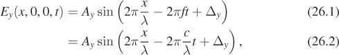
where Δy is a “phase” that depends on our choice of the origin of our coordinate system. Similarly, the z-component must have the form
Suppose we change units so that the speed of light, c, is 1.0; assume that λ = 1 as well, and Δz = 0. Plot Ez as a function of x when t = 0; do so again when t = 0.25, 0.5, 0.75, and 1.0.
Physical experiment confirms that the x-component of the electric field for a wave traveling on the x-axis is always zero. Thus, the vector a = [Ax Ay Az]T that characterizes the plane wave must always lie in the yz-plane; Ay and Az can take on any values, but Ax is always zero.
26.4.1. Diffraction
The first important phenomenon associated with the wave nature of light is diffraction. Just as waves passing through a gap in a breakwater fan out into a semicircular pattern, light waves passing through a small slit also fan out. Assuming the slit is aligned with the y-axis and the plane waves are moving in the x-direction, the electric field (after the light passes through the slit) will be aligned with the y-direction, that is, Az will be 0.
If we place an imaging plane at some distance from the slit (see Figure 26.7), a pattern of stripes indicating the wave nature of the light appears.
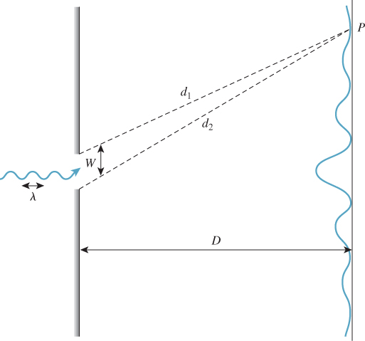
Figure 26.7: Light passing through a narrow slit spreads out to illuminate a surface behind the slit. Light from each side of the slit has different distances d1 and d2 to the back plane. When these distances are a half-wavelength apart, the light waves cancel; when they’re a multiple of a full-wave apart, they reinforce each other. This results in a set of bands of light and dark on the imaging plane with spacing approximately λD/w.
For the most part, this kind of diffraction effect is not evident in day-to-day life, but a closely related phenomenon, in which light of different wavelengths is reflected in different directions by some medium (things like the “eye” of a peacock feather, or a prism), is quite commonplace.
26.4.2. Polarization
In studying the electric field associated to light moving in the x-direction, we have a plane wave described by
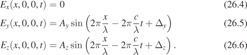
The phase constants Δy and Δz depend on where we choose the origin in x or t; if we replace x by x + a, then both Δy and Δz will change, but the difference between them will remain the same. This difference can be any value at all (mod 2π); in typical light emitted from an incandescent lamp, for instance, all possible differences between 0 and 2π are equally likely.
The simplest case is a plane wave where Ay = Az and Δy – Δz = π/2 or 3π/2. Such a wave is called circularly polarized. If we consider the electric field of Equation 26.6 at time t = 0 and assume that we’ve adjusted the x-axis so that Δy = 0 and Δz = π/2, the field has the form
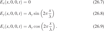
Notice that for every value of x, the vector E is a point on the circle of radius Ay in the yz-plane. Figure 26.8 shows this. We’ve plotted in blue the electric field along the x-axis at a fixed time t. The projection of this field to the xy-plane, shown in red, is sinusoidal. The projection to the xz-plane, in green, is also sinusoidal, with the same amplitude, because Ay = Az. The projection operation, for one vector, drawn in black, is shown by two magenta dashed lines. The projection of all these vectors to the yz-plane, shown in black, forms a circle in that plane.
What happens to the preceding analysis when Δy = 0 and Δz = – ![]() ? These two similar, but different, situations are called clockwise and counterclockwise polarization.
? These two similar, but different, situations are called clockwise and counterclockwise polarization.
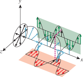
At the other extreme, consider the case where Δy = Δz = 0. In this case, the electric field vector at every point of the x-axis is a scalar multiple of [0 Ay Az]T, that is, the electric field vectors all lie in one line. Figure 26.9 shows this: The projections of these vectors to the yz-plane all lie in one line, determined by the numbers Ay and Az. Such a field is said to be linearly polarized, with the direction [0 Ay Az]T being the axis of polarization.
Finally (see Figure 26.10), there are cases where Δy – Δz is not a multiple of ![]() , or where Ay and Az differ. In this case, the projection of the field vectors to the yz-plane forms an ellipse, and the light is said to be elliptically polarized. It turns out that an elliptically polarized field can always be expressed as the sum of a circularly polarized one and a linearly polarized one, with the axis of linear polarization being along the major axis of the ellipse (see Exercise 26.11).
, or where Ay and Az differ. In this case, the projection of the field vectors to the yz-plane forms an ellipse, and the light is said to be elliptically polarized. It turns out that an elliptically polarized field can always be expressed as the sum of a circularly polarized one and a linearly polarized one, with the axis of linear polarization being along the major axis of the ellipse (see Exercise 26.11).

There are materials called polarizers that are transparent to waves of one polarization but opaque to those of the opposite polarization.
Light traveling in some direction d and reflected from a shiny surface with normal vector n, when reflected, ends up preferentially linearly polarized with the polarization direction being d × n. Such reflected light, when observed through a polarizer that favors light of some other polarization, will be attenuated. This is the principle by which polarized sunglasses filter reflected sunlight. The precise nature of reflected polarized light depends on the reflecting material, as we’ll see in Section 26.5.
26.4.3. Bending of Light at an Interface
In a related phenomenon, light passing from one medium to another changes speed. The speed of light in a vacuum is the highest possible speed; in other materials it may be substantially slower, due to the virtual transitions mentioned earlier. As a result, when light passes from a vacuum to some material it slows down. This does not affect the frequency of the light, that is, the number of peaks of electromagnetic radiation arriving at a fixed point in a fixed amount of time. You can convince yourself of this by observing a person who jumps into a swimming pool: The color of his or her clothing does not appear to change whether you’re seeing it through water and air or just air. The speed change does affect the wave length, however, which is determined by
λ = s/f,
where s is the speed of light in whatever medium it’s traveling through and f is the frequency.
The index of refraction or refractive index of a medium is the ratio of the speed of light in a vacuum to the speed of light in that medium. It’s denoted by the letter n. Typical indices of refraction are 1 for a vacuum, 1.0003 for air, 1.33 for water, and 2.42 for diamond.
The difference of refractive index in different media causes a macroscopic phenomenon: Light rays bend when they go from one medium to another. The conventional name for the precise description of the bending is Snell’s law, although the phenomenon of a consistent law of refraction was known to Ibn Sahl of Baghdad as early as 984 CE [Ras90].
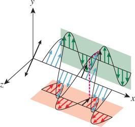
The bending follows a particularly simple form (see Figure 26.11): If θ1 and θ2 denote the angles between the ray and the surface normal on the two sides of the interface, and n1 and n2 denote the two indices of refraction, then
This tells us that if we know n1, n2, and θ1, we can determine θ2. The index of refraction, n, determines a great deal about how light interacts with a medium. For instance, when light arrives at the interface between air and glass at some angle, the refractive index determines not only the amount of bending, but also how much of the light is transmitted through the glass and how much is reflected, as we’ll see in Section 26.5. Those interested in physically realistic renderings of glass and other transparent materials must take this fact into account.
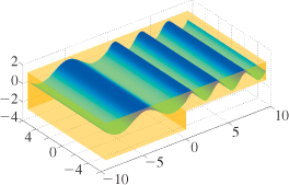
Using only the assumption that the electromagnetic field has a sinusoidal form with the same frequency in each medium, and is continuous, we can prove Snell’s law. Fortunately, the mathematics of this explanation apply to any kind of wave, not just plane waves in three dimensions, so we can illustrate the idea with linear waves in a plane. Consider the situation shown in Figure 26.12: a shallow tray whose left side is twice as deep as its right side; this makes waves on the left half travel about twice as fast as those on the right half. If we create sinusoidal waves of frequency f on the left side, moving right, when they enter the right side they “bunch up.” Because of the slower speed on the right, the same number of waves per second reach the right-hand side of the tray as reached the midline.
When we create waves traveling in an off-axis direction (see Figure 26.13) in the left half of the tank, they arrive at the dividing line between the two sides and continue on as waves in the shallower right-hand side of the tank. The peaks of the waves on the two sides of the tank must match up at the dividing line if the wave height is to be a continuous function; for this to happen, the directions of propagation must differ.
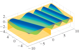
(a) Suppose that the wavelength of the waves in the left half of the tank is λ, and the direction of propagation in the left side is at angle θL ≠ 0 to the left-right axis of the tank. Show that along the midline of the tank, the distance between peaks is λ/ sin(θL).
(b) For a corresponding statement to be true on the right side of the tank, where the wavelength is about λ/2, the distance between peaks will be (λ/2)/ sin(θR). Setting these equal, show that sin(θL)/ sin(θR) = 2, which is exactly the ratio of the velocities in the two sides of the tank.
A similar phenomenon happens with plane waves that meet at a planar interface between media, from which Snell’s law follows as a consequence.
The index of refraction of a medium is not really a constant: It depends on the wavelength of the light. Cauchy developed an empirical approximation for the dependence, showing it was of the form
where the values of A and B are material-dependent. The exact values are not important, except that B ≠ 0. This means that light of different wavelengths, arriving at an interface between different media, gets bent by different amounts: The different wavelengths are separated from one another. One instance of this is the rainbows cast by prisms when they are struck by sunlight. Another is that lenses, which are supposed to focus light at a single point, actually focus light of different wavelengths at different points: When red light is in focus, blue light will be blurry, etc. This chromatic aberration is a significant problem in lens design, and many lens coatings are designed to minimize it.
26.5. Fresnel’s Law and Polarization
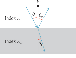
Consider Figure 26.14, which shows light arriving at the interface between two media, the upper (y > 0) having refractive index n1 and the lower (y < 0) having index n2. For now, we’ll assume that the media are insulators rather than conductors. The light’s direction of propagation lies in the xy-plane, the plane of the diagram. The arriving light makes angle θi (“i” is for “incoming”) with the y-axis; the reflected light makes angle θr = θi, and the transmitted light makes angle θt with the negative y-axis. Since the electric field associated to the incoming light must be perpendicular to the direction of propagation, we’ll consider two special cases. In the first, the electric field, at each point of the incoming ray, points along the z-direction (i.e., parallel to the interface between the media, pointing either into or out of the page). A light source with this property is said to have “parallel” polarization with respect to the surface, or be p-polarized.
When such a wave reaches the surface the electric field interacts with the electrons near the interface, moving them back and forth in the z-direction; these motions in turn generate a new electromagnetic field that’s a sum of two parallel-polarized waves, the first corresponding to the transmitted light and the second to the reflected light. The transmitted light travels in a direction described by Snell’s law, and the reflected light travels according to the familiar “angle of incidence equals angle of reflection” rule: θr = θi. The fraction Rp of light reflected depends on the angle θi according to the rule
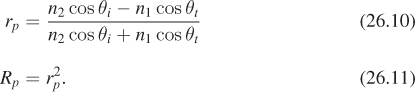
the fraction transmitted Tp is just 1 – Rp. (These fractions denote the fraction of the incoming power that leaves in each direction. The amplitude of the reflected wave is just rp times the amplitude of the arriving wave.) These formulas can be derived, like Snell’s law, by insisting on continuity at the interface [Cra68].
The phase of the reflected light may match that of the arriving light, lag behind it, or lead it, or be 180° out of phase with it.
The other special case is when the electric field is perpendicular to the z-axis, that is, it lies entirely in the xy-plane, perpendicular to the direction of propagation. Such a wave is said to be s-polarized. In this case, the reflection coefficient Rs is given by
Once again, the transmission coefficient Ts is 1 – Rs. These rules for the reflection and transmission coefficients for s- and p-polarized waves are called the Fresnel equations, after Augustin-Jean Fresnel (1788–1827).
Because every wave can be written as a sum of an s-polarized and a p-polarized wave, these two special cases in fact tell the whole story. For instance, incoming light that is linearly polarized as the sum of a wave that is equal parts s-polarized and p-polarized will reflect and again be linearly polarized. But the ratio of s- to p-polarized components will no longer be one to one; instead it will be Rs/Rp. Because in general Rs > Rp, the reflected light will be more s-polarized than the incoming light. In fact, no matter what the mix of s- and p-polarized light in the arriving light, the outgoing light will be more s-polarized than was the incoming light. The same argument applies to circularly polarized light; the only difference is one of phase, which does not enter the Fresnel equations. Incoming circularly polarized light will generally reflect into elliptically polarized light, with the s-component dominating.
(a) For n1 = 1 and n2 = 1.5 (corresponding approximately to air and glass), plot Rp against θi, and observe that at about 56°, Rp is 0; what does this tell you about the polarization of the reflected light when light arrives at this angle?
(b) For any pair of materials, there’s a corresponding angle; it’s called Brewster’s angle. Briefly explain why Brewster’s angle depends only on the ratio of the indices of refraction of the materials.
Consider light traveling from a piece of glass to the air (so n1 = 1.5 and n2 = 1.0). Plot Rs and Rp against θi for 0 ≤ θi < sin–1(n2/n1) ≈ sin–1 (.66). At the upper end of this range, the critical angle, both Rs and Rp are 1; all light is reflected back into the glass and none escapes to the air. This is called total internal reflection.
Figure 26.15 demonstrates Fresnel’s law. The first photo shows several coins and a washer in a tray as seen from above on a calm, overcast day. The second shows the same items, seen from about 45°. So much of the incident light is reflecting that it’s much more difficult to see the items in the tray.
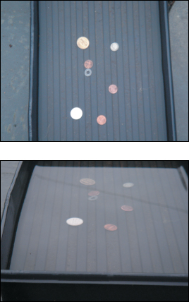
Figure 26.15: Fresnel’s law in action: The coins are easily visible from overhead, but are obscured by sky reflections when seen at a diagonal.
The analysis above applies to insulators. For conductors, the transmitted light is almost immediately absorbed, and the rate at which it’s absorbed has an effect on the reflected light. One analysis revises the index of refraction to be a complex constant, whose real and imaginary parts correspond to the usual index of refraction and the amount of absorption in the material, known as the coefficient of extinction and denoted κ. An alternative approach simply treats the refractive index and coefficient of extinction as separate quantities. In this latter form, a good approximation to the Fresnel reflectance for conductors (in air) is given by
where n2 is the index of refraction of the metal and κ is its coefficient of extinction.
Snell’s and Fresnel’s laws are quite general, but there are materials whose behavior is more interesting than that described by these equations. Calcite, for instance, exhibits birefringence, in which there are two directions of refraction rather than one; so does topaz. (That’s because the speed of light is different in different directions through these materials!)
26.5.1. Radiance Computations and an “Unpolarized” Form of Fresnel’s Equations
While Fresnel’s laws describe transmitted and reflected power, in graphics we’re mostly concerned with radiance, which we’ll define in the next few sections. Because radiance involves an angle measure in its definition, and the angle between two light beams refracted by Snell’s law is different before and after refraction, the ratio between outgoing and incoming radiance involves an extra factor of
The derivation of this factor is given in the web materials for this chapter.
Although we’ve observed that light, after reflection, tends to be increasingly polarized, it’s common in graphics to treat light as unpolarized, that is, to assume that the polarization of incident light is, on average, zero. With that assumption, the Fresnel equations can be simplified to a single factor, called the Fresnel reflectance, which is
The energy reflected is RF times the incident energy. And the energy transmitted is (1–RF) times the incident energy. This means that the reflected and transmitted radiance values can be computed as
Note that RF here depends implicitly on θi, n1, and n2 which, together with Snell’s law, lets us compute θt.
26.6. Modeling Light as a Continuous Flow
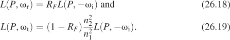
Imagine standing at a crossroads, looking north. You count the cars that come to the crossroads from the north, and observe that 60 cars arrive in the course of an hour. You report that the arrival rate for cars is 60 per hour, and this lets you guess that in 10 minutes, about 10 cars will arrive; in 5 minutes 5 cars will arrive, etc. Of course, at an actual crossroads, cars arrive irregularly, so your “5 cars in 5 minutes” claim is probably not exactly correct. Nonetheless, if you counted cars for each hour over the course of the day, you could make a graph like the one shown in Figure 26.16, where we’ve connected the dots with straight lines, but could have used a smooth curve. Later you could say something like “the arrival rate at 9:30 was about 65 cars per hour.”
In making such a statement, you are treating the arrival rate as something that makes sense at a particular instant; you are treating this problem as if it were continuous rather than discrete so that the tools of calculus (e.g., instantaneous rates) actually apply to it, while in fact only finite-time rate measurements (“19 cars arrived between 9:20 and 9:43”) make sense.
We’ll do the same thing with light. As we observe the light arriving at a small piece of surface, we can think of ourselves as counting “arriving photons over some period of time.” But instead we treat the light as if it were infinitely divisible, and talk about instantaneous rates of light arrival. In fact, rather than counting photons, we’ll count the arriving energy, because photons of different wavelengths have different energies, but the idea remains the same.
This assumption that there is an instantaneous rate of energy arrival at a surface lets us use calculus to talk about light energy. We’ll repeat this “limiting trick” twice more, once to establish a rate of arrival per area as we consider smaller and smaller areas, and again to consider the rate of energy arriving from a particular set of directions, divided by the size of that set of directions, as the size of the set goes to zero. Having described this quantity (which we’ll call radiance), we’ll see that all practical measurements we can make can be expressed as integrals of radiance over various areas, time periods, and sets of directions. The abstract entity, radiance, turns out to be easy to work with using calculus, and all the things we can measure are integrals of radiance.
In this discussion so far, we’ve moved from a discrete version of counting to one in which the light-energy arrival rate is continuous. We’ll now do the same thing in two more ways, with respect to angle and area.
26.6.1. A Brief Introduction to Probability Densities
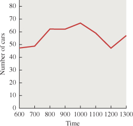
Before we do so, let’s look at a related concept from probability theory, the notion of probability density. Consider a random number generator that randomly generates real numbers between 0 and 5. We observe 1,000 of these randomly generated real numbers, and look at how many lie between 0 and 0.5, between 0.5 and 1.0, etc. The resultant histogram (see Figure 26.17) looks fairly smooth; looking at it we might conjecture that the random number generator is uniform, in the sense that every number is equally likely to be generated. But if we choose smaller bins to count—say, between 0 and 0.001, between 0.0001 and 0.0002, etc.—the uniformity is no longer so obvious. Indeed, the probability of generating any particular random number must be zero. Thus, when we are discussing probabilities where the domain is some interval in the reals (rather than a discrete set, like the set of faces on a pair of dice), we talk not of the probabilities of generating particular numbers, but of generating numbers within an interval [a, b]. If the generator really is generating numbers uniformly, then the probability of generating a number in the interval [a, b] is proportional to b – a. More generally, we posit the existence of a function p : [0, 5] ![]() R called the probability density function or pdf with the property that
R called the probability density function or pdf with the property that
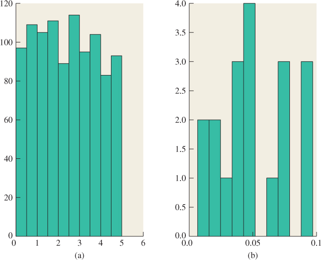
Figure 26.17: (a) A histogram of 1000 random numbers between 0 and 5, in bins of width 1/2; the distribution appears to be uniform. (b) A portion of a finer histogram, with bins of size 0. 01; at this scale, it’s not clear that the distribution is uniform.
For the uniform distribution on the interval [0, 5], p is the constant function with value 1/5. For other distributions, p is not constant. But because its integral represents a probability, p must be everywhere nonnegative, and its integral over [0, 5] must be 1. 0.
An alternative formulation for describing a distribution is the cumulative distribution function or cdf, defined by
If F is continuous and differentiable, then the two formulations are related by noting that p = F′. The big advantage of the cdf formulation is that probability masses can be incorporated easily, that is, single points in the real line at which a nonzero amount of probability is concentrated. At a point b where there is a probability mass, there’s also a discontinuity in the cdf, with the “jump” being exactly the probability mass at b. The student who wishes to work carefully with the “impulses” that arise in the geometric optics description of mirror reflection and refraction, and which correspond exactly to the notion of probability masses, will do well to study the cdf approach to defining distributions.
Verify that the function 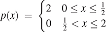 is a probability distribution on [0, 2]. Notice that p(0.5) = 2, but this does not mean that the chance of picking 0.5 as a sample from this distribution is 2. We see from this example that while probabilities may not exceed 1.0, probability densities may.
26.6.2. Further Light Modeling
Now we return to the crossroads. Just as cars arrive from the north at a certain rate, other cars arrive from the south, the east, and the west. To adequately describe all the arriving cars requires you to keep multiple tallies, one for each arrival direction. If the crossroads were a more complex intersection, with five, or six, or ten roads leading into it, you’d need more and more tallies. If cars could arrive in any direction, then in the analogy with the probability densities we just discussed the probability of a car arriving from any particular direction would be zero. Instead, we’d have to talk about a density, where the probability of a car arriving from a range of directions was gotten by integrating the density over that range of directions.
Analogously, light energy can arrive at a point from any direction. The amount arriving from a range of directions depends in part on how large the range is: If you narrow the range of directions, you observe less incoming light energy. Indeed, if you narrow your range of directions to a single direction, no energy at all will arrive from that direction. We speak, therefore, of a density, where the amount of energy arriving in some range of directions is gotten by integrating this density over that range of directions.
Just as the energy from a single direction is zero, the energy arriving at any single point is also zero. To get something meaningful, we must consider the energy arriving over some small region. Once again, this is done with a density: We posit a function whose integral, over a small region,1 gives the amount of energy arriving there.
1. We’ll generally use the term “region” to indicate a portion of a surface, and the term “area” to indicate the size of that region (i.e., something whose units are m2), although we’ll occasionally use terms like “pixel area” to indicate a region.
All of this will be made more explicit in Section 26.7; for now the key idea is that our model of light moving around in a scene will be based on a density function whose arguments range over several continua: time, position, and direction.
26.6.3. Angles and Solid Angles
To define a “range of directions” for light arriving at a surface in 3-space, we need to define a notion of “solid angle” in R3 in analogy with the notion of angle in R2.
An angle in R2 is usually defined by a pair of rays at a point P (see Figure 26.18). If we look at a unit circle C around P, there’s an arc A contained between the rays. The length of the arc A is the measure of the angle.
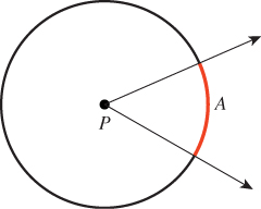
We can revise this definition slightly, and say that the arc A is the angle. Clearly, if you know the arc A and the point P, you can find the two rays, and vice versa, so the distinction is a small one. But we can then generalize, and say that an angle at P is any subset2 of the unit circle C at P. The measure of the angle is the total length of all the pieces of the subset. In practice, there are typically a finite number of pieces—usually just one—so this isn’t a large generalization. Finally, it’s often convenient to not talk about points of the circle C, but about points on the unit circle, or unit vectors. For any point X in C, we can form the unit vector v = X – P. Given v and P, it’s easy to recover X = P + v. So our revised notion of an “angle at P” is this: An angle at P is either a subset of the unit circle C with center P, or a subset of the set S1 of all unit vectors.
2. ![]() Any measurable subset [Roy88]. See Chapter 30.
Any measurable subset [Roy88]. See Chapter 30.
The notions of “clockwise” and “counterclockwise” angles, and “the angle from ray1 to ray2” (which might be much larger than π) and of angles that “wrap around multiple times” can all be defined with careful adjustments of the definition above; in our study of light, though, we’ll have no need for these ideas, so we’ll simply use the definition of angle and measure above.
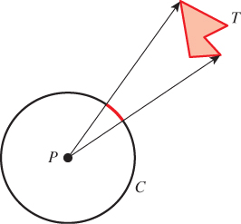
One common use of angles is the notion of the angle subtended by some shape, T, at a point P (see Figure 26.19). The shape T is projected onto the unit circle C around P, and the measure of the resultant angle is called the angle sub-tended by T at P. In equations, the angle subtended by T at P is
We can now describe solid angles in R3 by analogy. A solid angle at a point P ![]() R3 is a (measurable) subset Ω of the unit sphere about P, or, equivalently, a measurable subset of S2, the collection of all unit vectors in 3-space. The measure of the solid angle of Ω is the area of the set Ω (see Figure 26.20).
R3 is a (measurable) subset Ω of the unit sphere about P, or, equivalently, a measurable subset of S2, the collection of all unit vectors in 3-space. The measure of the solid angle of Ω is the area of the set Ω (see Figure 26.20).
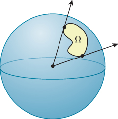
Figure 26.20: The solid angle Ω is a set on the surface of the unit sphere. The measure of the solid angle is the area of this set.
When we want to treat points in a solid angle as unit vectors, we’ll use bold Greek letters, almost always using the letter ω. We’ll often write “Let ω ![]() Ω ...”, and thereafter treat ω as a unit vector, writing expressions like ω · n to compute the length of the projection of a vector n onto ω. In fact, this use of a solid angle as a collection of direction vectors is almost the only one we’ll see.
Ω ...”, and thereafter treat ω as a unit vector, writing expressions like ω · n to compute the length of the projection of a vector n onto ω. In fact, this use of a solid angle as a collection of direction vectors is almost the only one we’ll see.
The notion of subtended angle can also be extended to three dimensions: If T is a shape in R3 and P a point of R3 with P ![]() T, the solid angle subtended by T at P is the area of the radial projection of T onto the unit sphere at P, in exact analogy with the two-dimensional case. More precisely, the solid angle subtended by T at P is
T, the solid angle subtended by T at P is the area of the radial projection of T onto the unit sphere at P, in exact analogy with the two-dimensional case. More precisely, the solid angle subtended by T at P is
{S(Q-P) : Q ![]() T},
T},
in exact analogy with the 2D case.
This definition lets us speak of “solid angles” on other spheres (e.g., like the Earth) by defining their measure to be the measure of the solid angle they subtend at the center of the sphere. It’s easy to show that if U is a subset of a sphere of radius r about P, and the area of U is A, then the solid angle represented by U (i.e., the solid angle subtended by U at P) is A/r2. When we speak of measuring a solid angle on some arbitrary sphere (like the Earth, or a spherical lightbulb), it is implicit that we mean “the solid angle subtended at the center of the sphere by this region.”
Estimate the solid angle measure of your country as a solid angle on the (roughly) spherical earth. Use 13,000 km (or 8000 mi) as the diameter of the Earth.
Notation: It’s conventional to use Ω to denote both a solid angle and the measure of that solid angle (just as we use θ to denote an angle and its measure in the plane). Just as we often use x as a variable of integration in calculus, it’s common to use the letter Ω to denote a solid angle, and ω to denote a member of Ω, so that ω is a unit vector.
Units: Just as angles are measured in radians, solid angles are measured in steradians, abbreviated “sr.” The entire unit sphere has a solid angle measure of 4π steradians.
26.6.4. Computations with Solid Angles
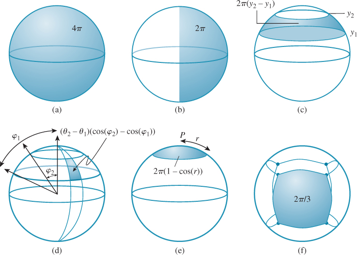
Let’s now measure a few simple solid angles (see Figure 26.21). Following the standard from graphics rather than mathematics, we will treat the y-axis as pointing up, the x-axis as pointing to the right, and the z-axis as pointing toward us. Thus, the longitude is atan2(y, z) and the latitude is arcsin(y). (The colatitude, which is often denoted φ in spherical polar coordinates, is arccos(y). The other polar coordinate, θ, is what we’ve called the longitude.)
• If Ω is all of S2, then the measure of Ω is 4π (the area of a unit sphere).
• Any hemisphere has measure 2π.
• The “stripe” between y = y0 and y = y1 has area 2π ||y1 – y0||. This follows from the theorem below, as do the next two examples.
• The latitude-longitude rectangle between latitudes λ0 and λ1 and longitudes θ0 and θ1 has solid angle ||θ1 – θ0|| · ||sin λ1 – sin λ0|| (where latitude goes from –π/2 at the South Pole to π/2 at the North Pole). (When the longitudes are on opposite sides of the international dateline, this rectangle is a very long stripe wrapping around the nondateline part of the globe.)
• A “disk” consisting of all points whose spherical distance from a point P is less than r (where r < π) has solid angle measure 2π(1 – cos(r)).
• If a regular solid of n sides (cube (n = 6), tetrahedron (n = 4), octahedron (n = 8), dodecahedron (n = 12), icosahedron (n = 20)) is inscribed in the unit sphere, the projection of one of its faces onto the sphere (see Figure 26.21 (f)) has solid angle measure ![]() , because the total projected area is 4π, and by symmetry, each face has the same projected area.
, because the total projected area is 4π, and by symmetry, each face has the same projected area.
All of the results above are consequences of the sphere-to-cylinder projection theorem: If C is a cylinder of radius 1 and height 2, circumscribed about the sphere S of radius 1, then the horizontal radial projection map,
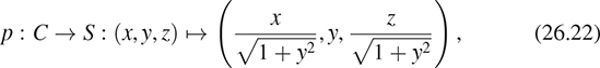
is area-preserving. (The proof is a simple calculus computation—see Exercise 26.1). Figure 26.22 shows this: The area of a country on the surface of the globe is the same as the area on the plate carrée projection shown (although many other characteristics of shape are grossly distorted, as shown for Greenland [in green]).
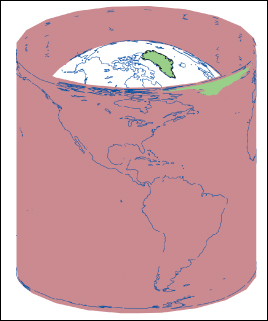
Figure 26.22: Horizontal radial projection from the sphere to the surrounding cylinder is area-preserving.
As an example of another use of this theorem, let’s let Ω denote the northern hemisphere y ≥ 0 of the unit sphere, and integrate the function y over this hemisphere.
That is to say, we seek to evaluate
Consider the upper half-cylinder H = {(x, y, z) : x2 + z2 = 1, 0 ≤ y ≤ 1}, which projects to Ω under the axial projection map p. We can perform a change of variables in the integral, and express B as
where (x, y, z) = p(x′, y′, z′), and dA′ is area on H, and |Jp| is the Jacobian for the change of variables (i.e., it represents how areas at (x′, y′, z′) are stretched or contracted to become areas at (x, y, z)). The theorem that p is area-preserving means that |Jp| = 1, so the integral becomes
Since in the formula for p, y does not change, we have y = y′, so this becomes
By circular symmetry, this is just 2π times the integral of y′ from 0 to 1. That integral is 1/2, so B = ![]() · 2π = π.
· 2π = π.
If instead we wanted to know the average of y over the upper hemisphere, we’d need to divide its integral (π) by the area of the hemisphere (2π). The average is thus ![]() . This value comes up often, although it’s usually in a slightly generalized form: We have a hemisphere defined by ω · n ≥ 0, and we want to know the average value of ω · n over this hemisphere. (Our instance is the special case where n = [0 1 0]T.) We’ll state this as a principle:
. This value comes up often, although it’s usually in a slightly generalized form: We have a hemisphere defined by ω · n ≥ 0, and we want to know the average value of ω · n over this hemisphere. (Our instance is the special case where n = [0 1 0]T.) We’ll state this as a principle:
The average height of a point on the upper hemisphere of the unit sphere is ![]() . Thus, for any unit vector n, the integral
. Thus, for any unit vector n, the integral
In various computations, one has both a solid angle Ω in the sphere S around a point P, and a surface M containing P, which can be locally thought of as a plane K through P (namely, the tangent plane to M at P). The projected solid angle Ω is the area of the projection of Ω onto the plane K (see Figure 26.23).
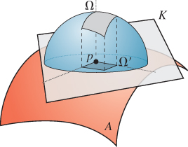
Figure 26.23: For a solid angle Ω in the unit sphere around a point p of a surface M, the projected solid angle lies in a plane K tangent to M at p. The projected solid angle Ω will always have a smaller area than the original solid angle.
(a) What is the largest possible projected solid angle for any solid angle Ω in a hemisphere bounded on one side by the plane K?
(b) For the case where P is the origin and K is the xz-plane, compute the projected solid angle of the “positive x quadrant” (the points of S with x, y ≥ 0).
(c) Do the same for the region consisting of all points with latitude greater than 30° north (i.e., approximately the northern extra-tropical zone).
(d) Show that the solid angles of the two regions are the same.
(e) Explain why the projected solid angles are different.
(f) Compute the projected solid angle of the region θ0 ≤ θ ≤ θ1, φ0 ≤ φ ≤ φ1, where φ0 and φ1 are both between 0 and π/2, that is, the projected solid angle of a small latitude-longitude patch in the upper hemisphere. Hint: You should be able to answer every part of this question without computing any integrals; the sphere-to-cylinder projection theorem will help.
26.6.5. An Important Change of Variables
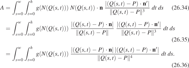
Often in the next several chapters we’ll have occasion to integrate some function over the solid angle Ω subtended by some rectangle R, of width w and height h, at a point P, as shown in Figure 26.24. Usually this function involves a factor of ωi · n, where n is the surface normal at P and ωi ![]() Ω is the variable of integration, in which case the integral looks like
Ω is the variable of integration, in which case the integral looks like
In some cases involving transparency, the ωi · n factor will be negative and will require absolute value signs.
Expressing Ω in terms of latitude and longitude, or even in terms of xyz-coordinates, may be extremely messy. It’s often convenient to perform a change of variables instead, and integrate over the rectangle R. We’ll carry this out for the particular case where P is the origin so that the mapping from a point (x, y, z) on R to a point on the unit sphere has a particularly nice form:
(We’ve chosen the letter N here for “normalize.”)
The change of variables formula says that to compute
we can instead compute
where JN is the Jacobian for the change of variables N.
Let’s suppose that the rectangle R is specified by a corner, C, and two perpendicular unit vectors u and v, chosen so their cross product n′ points back toward P. The points of R are then of the form
Q = C + su + tv,
where 0 ≤ s ≤ w and 0 ≤ t ≤ h. So the integral we need to compute is

Computing the Jacobian of N at the point Q = C + su + tv is somewhat involved, but the end result is simple:
where r is the distance from P to Q and ω is the unit vector pointing from P to Q.
The intuitive explanation for this is that if the plane of the rectangle R happened to be perpendicular to ω, then a tiny rectangle on R, when projected down to the unit sphere around P, would be scaled down by a factor of r in both width and height, and that accounts for the r2 in the denominator. If the plane of R is tilted relative to ω, then we can first project the tiny rectangle onto a plane that’s not tilted (projecting along ω). This, by the Tilting principle, introduces a cosine factor, which is ω · n′.
Applying this result to the point Q(s, t) = C + su + tv, the integral A becomes
If we define ![]() , this simplifies to
, this simplifies to

To make this concrete, Listing 26.1 shows how you might actually estimate this integral numerically, given the function g that takes a unit vector as an argument.
Listing 26.1: Integrating a cosine-weighted function over the solid angle subtended by a light source.
1 // Given rectangle information C (corner), u, v (unit edge vectors),
2 // w, h (width and height) and n' (unit normal), a point P on
3 // a plane whose normal is n, and a function g(.) of a single
4 // unit-vector argument, estimate the
5 // integral of g(ω)ω·n over the set Ω of
6 // directions from P to points on the rectangle.
7
8
9 sum = 0;
10 for i = 0 to N-1
11 s = i/(N-1)
12 Δs = 1/(N-1);
13 for j = 0 to N-1
14 t = j/(N-1)
15 Δt = 1/(N-1)
16 Q = C + s * u + t * v
17 ω = S(Q - P)
18 r = ‖Q - P‖
19
20 ![]()
21
22 return sum
To summarize, when we change from an integral over solid angles to an integral over some planar surface with normal n′, we introduce an extra factor in the integrand, of the form ![]() , where ω is the unit vector from P to a point Q on the surface and r is the distance from P to Q. Often the integrand will already have the form g(ω)|ω · n|, so the integrand for the area integral will be
, where ω is the unit vector from P to a point Q on the surface and r is the distance from P to Q. Often the integrand will already have the form g(ω)|ω · n|, so the integrand for the area integral will be
26.7. Measuring Light
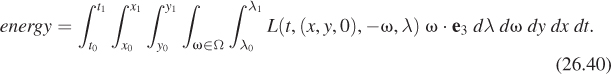
With the notion of solid angle in hand, we can now precisely describe how light energy is flowing in a scene. We’ll consider a function L, called the spectral radiance. It’s a function of time, position, direction, and wavelength that captures the infinitesimal characteristics of light transport in the sense that when it’s integrated over a time interval, and over some part of a surface perpendicular to the direction of transport, and over some solid angle of directions, and over some range of wavelengths, the result is the total light energy that arrives at that surface, arriving from the specified directions, within the range of wavelengths, and during the time interval. We previously discussed summing up energies for all different wavelengths, and we’ll do that presently, but for now, we want to consider the per-wavelength function—yet another density!
The integral of spectral radiance over a small surface, and a small range of directions, and a small period of time, and a small range of wavelengths, is the sort of thing that can be measured by a physical device, while the infinitesimal version is the thing that’s easy to work with mathematically, just as it’s possible to measure the distance a car travels over some small time interval, but we work with instantaneous velocity when we’re studying the mathematics of motion. What are the units of L? Taking as a model “piece of surface” a rectangle in the xy-plane, and assuming that the light flow is in a set of directions Ω all of which are essentially perpendicular to the xy-plane, we know that

Note that in the integrand above, L has four arguments: t, the point (x, y,0), – ω, and λ. The ω is negated because ω points out of the surface, but we want to sum up the light coming in to the surface.
Using MKS units for the surface and time, but nanometers for wavelength (which follows long-standing convention), we find that L must have the units of joules per second per square meter per nanometer per steradian. One joule per second is one watt, so we can also say “watts per square-meter nanometer steradian.”
What happens if the direction ω along which light arrives is not parallel to the surface normal? Then the amount of light energy arriving at the surface, per unit area, is smaller than if it were parallel, by the Tilting principle.
Thus, the more general and exact formula for the energy arriving at that small region of the xy-plane from directions in the solid angle Ω, in the given time interval and wavelength interval, is
For a region R of an arbitrary plane, with normal vector n, the energy arriving at R in the interval t0 ≤ t ≤ t1, at wavelengths λ0 ≤ λ ≤ λ1, in directions opposite those in a solid angle Ω, is

where ∫P![]() R ... dP is an area integral over the area R.
R ... dP is an area integral over the area R.
When we are concerned with overall light energy, rather than caring about how much is transported at each different wavelength, we can integrate L over all wavelengths λ, giving us a new function depending on time, position, and direction, with units of watts per square-meter steradian. This new function is called the radiance. This relationship between spectral radiance and radiance is quite general: For any photometric quantity, the spectral version has the wavelength λ as a parameter, while the version without the adjective “spectral” has been integrated over all possible wavelengths.
The function L, defined for all times and points and all directions (and possibly for all wavelengths) describes fully the way light flows around the scene. We’ll call L(t, P, ω) or L(t, P, ω, λ) the “radiance” or “spectral radiance” at time t, location P, etc. But the function L, considered as a whole, is sometimes also called the plenoptic function, particularly in computer vision.
26.7.1. Radiometric Terms
The spectral radiance L characterizes the light energy flowing, at each instant, at each point in the world, in each possible direction. Formally its domain is
R × R3 × S2 × R+,
where S2 denotes the unit sphere in 3-space (the set of all possible directions in which light can flow) and R+ is used for the set of all possible wavelengths. In practice, R+ may be replaced by the range of wavelengths that are visible. The codomain of L is R.
Starting from L, we can describe, via integration, all of the terms conventionally used in radiometry, the science of the measurement of radiant energy. An alternative approach is to start from energy or power, and define all the terms by differentiation. We discuss this approach briefly in Section 26.9.
26.7.2. Radiance
Spectral radiance is the quantity described by L; radiance is the quantity
which is defined for (t, P, ω) ![]() R × R3 × S2. In engineering, the letter L is usually used for this quantity, with Lλ being reserved for spectral radiance; in graphics, however, the spectral radiance is often denoted by L. Because for us the symbol λ actually is one of the arguments to the function, it’s a bad choice for a subscript. We’ll therefore carry out the remainder of this discussion in the spectral case (keeping λ as an argument), and discuss the nonspectral case at the end. Until then, when we speak of radiance we’ll be speaking of spectral radiance; when we speak of irradiance we’ll mean spectral irradiance, etc.
R × R3 × S2. In engineering, the letter L is usually used for this quantity, with Lλ being reserved for spectral radiance; in graphics, however, the spectral radiance is often denoted by L. Because for us the symbol λ actually is one of the arguments to the function, it’s a bad choice for a subscript. We’ll therefore carry out the remainder of this discussion in the spectral case (keeping λ as an argument), and discuss the nonspectral case at the end. Until then, when we speak of radiance we’ll be speaking of spectral radiance; when we speak of irradiance we’ll mean spectral irradiance, etc.
The most interesting thing about radiance, from a computer graphics point of view, is that in a steady-state situation, that is, one in which L is independent of t, radiance is constant along rays in empty space (assuming, for the moment, that there are no point light sources; see Exercise 26.3). In mathematical terms, this means that the function L cannot be just any function. We also know, from physical considerations, that L can never be negative.
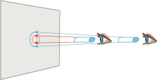
Why is L constant along rays in empty space? Try an experiment (see Figure 26.25): Look through a narrow cardboard tube at a tiny region of a well-lit latex-painted wall. You’ll see a small disk of light at the end of the tube, outlined in red in the figure. Now move twice as far away from the wall, and look again at the same region. Again, you’ll see a small disk of light (outlined by the larger blue circle), and it will appear equally bright (assuming that the wall is about equally well lit over the region where you’re looking). There’s an easy explanation for this: When at first you were at distance r from the wall, light leaving the wall spread out to illuminate a hemisphere of radius r; when you move to distance 2r, it’s illuminating a hemisphere of radius 2r, whose area is four times as great. But as you look through your tube, you see four times as large a region of the wall. Hence the total energy coming down the tube toward your eye is constant. In each case, the light energy passing through the eye end of the tube is approximately the integral of the radiance over the region of the tube end. Because we’re assuming the wall is uniformly lit, this is just the (approximately constant) radiance times the area of the tube end times the solid angle subtended at the eye by the far end of the tube. The fact that things look the same means that the radiance has not changed as you moved along the ray from the wall to your initial eyepoint.
To the degree that the pixel area on the sensor in a digital camera can be regarded as infinitesimal (or that the variation of radiance with position on the sensor can be assumed small) and the solid angle of rays that hit that pixel can be considered infinitesimal (or the variation with direction assumed small), the response of the sensor (assuming it responds to total arriving energy) is proportional to radiance. In fact, high-quality cameras used for computer-vision experiments produce images whose individual entries are radiance values. To be more precise, the values they produce are often integrals, with respect to wavelength, of spectral radiance multiplied by a response function that characterizes how the sensor responds to radiance of each wavelength.
26.7.3. Two Radiance Computations
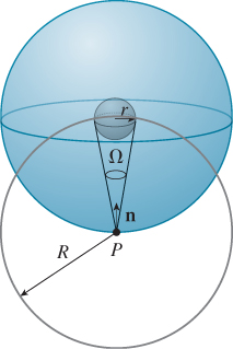
For a Lambertian emitter, the radiance in all outgoing directions is the same. Let’s suppose that we have a Lambertian emitting sphere S of radius r, emitting total power Φ. We’ll now compute the radiance along each ray leaving the sphere. The idea (see Figure 26.26) is to surround the emitter with a concentric sphere S′ of radius R >> r. All power emitted from S must arrive at S′, and the arriving power density (in W m–2) on S′ is independent of position. If we call this density D, then
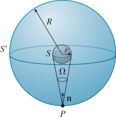
Figure 26.26: A radiating sphere inside a large receiving sphere. We’ll compute arriving power density at P.
We’ll compute the power density at the point P in terms of the unknown constant emitted radiance L, which will allow us to solve for L in terms of Φ. The power density at P is
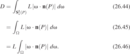
The transition between Equations 26.44 and 26.45 is justified by noting that for ω outside Ω, the radiance at P in direction –ω is zero, so the integral over the whole hemisphere can be reduced to an integral over just Ω.
For sufficiently large values of R, ω ·n(P) is very close to 1, so in the limit as R approaches infinity, we get
The sphere of radius R around P (drawn in light gray in Figure 26.27) has total area 4πR2, and subtends a solid angle of 4π at P; of this 4πR2 area, an area of approximately πr2 is occupied by the radiating sphere (i.e., as seen from P, the radiating sphere occludes a disk of area πr2 in the entire 4πR2). The solid angle subtended by the small sphere is therefore
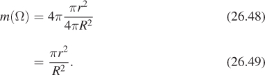
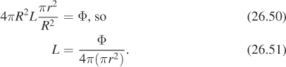
Substituting this in Equations 26.47 and 26.43, we get
We’ve made two approximations in this computation: that the dot product is always 1, and that the area occluded by the emitting sphere is πr2. If you instead evaluate the integral exactly, you’ll see that the two approximations exactly cancel each other.
We’ll now consider a similar example and analysis. This time we have a small disk-shaped emitter of radius r, that emits light only on one side (see Figure 26.28).
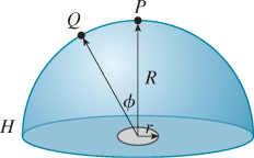
We enclose it in a hemisphere H of radius R, and first compute the power density at the North Pole P just as before; once again the power density is
At a point like Q that’s off-axis by the angle φ, the Tilting principle applies, and the power density arriving at Q is only cos φ times that arriving at P. Thus, the total power arriving at all points of the hemisphere (which must be the total emitted power Φ) is
by pulling the constant out of the integral. Further simplifying,
because the area of H is R2 times that of ![]() . Finally, by the Average height principle, we get
. Finally, by the Average height principle, we get
so that
This generalizes to arbitrary emitter shapes; in general, a one-sided planar Lambertian emitter of power Φ and area A emits light of radiance
26.7.4. Irradiance
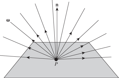
Irradiance is the density (with respect to area, time, and wavelength) of the light energy arriving at a surface from all directions. (It’s often described as the measure of the light hitting a surface “independent of direction,” but if the light energy varies with direction, then the meaning of that phrase isn’t entirely clear.) Irradiance is a useful notion when the surface is known to respond to incoming light in a way that’s direction-independent, where “respond to” might mean “absorb” or “reflect.” In cases where the response is direction-dependent, irradiance is generally irrelevant: Knowing only the total light energy hitting a surface will tell you nothing certain about the reflected energy.
Irradiance is usually defined only for a point P on a surface in the scene (or on a surface of some sensor like that of a virtual camera), and typically for a point where only reflective scattering takes place, that is, where there’s no transmission through the surface, so we need only consider light arriving from one side of the surface. Equation 26.42 says that the energy arriving at a region R from directions opposite those in a solid angle Ω is

The solid angle that interests us is ![]() (P) = {ω : ω · n(P) ≥ 0}, the set of all outgoing directions at P. So the irradiance at a point P where the surface normal is n is the innermost integral, using
(P) = {ω : ω · n(P) ≥ 0}, the set of all outgoing directions at P. So the irradiance at a point P where the surface normal is n is the innermost integral, using ![]() (P) as Ω. Within that integral, the dot product is always positive, so we can drop the absolute value signs,
(P) as Ω. Within that integral, the dot product is always positive, so we can drop the absolute value signs,
where we’ve substituted ωi for ω (see Figure 26.29).
This definition introduces some notational conventions we’ll follow for the next several chapters. First, P typically denotes a point on some surface in the
scene, while n(P) denotes the unit surface normal at P. The set of all “outward” vectors at P is ![]() (P), that is,
(P), that is,
We’ll sometimes generalize this and write
for the “positive hemisphere with respect to some vector n.”
Second, ωi is a vector pointing in this outward hemisphere toward some source of light, so the radiance reaching P from this source is L(t, P, –ωi, λ). The negative sign is important: ωi points toward the light source, but light flows from the source toward P, hence in direction –ωi. The “i” in ωi is a mnemonic for “incoming” rather than an index, which is why it is typeset in roman rather than italic. We’ll also often use ωo, a direction in which light leaves from P (often toward the observer’s eye).
The units of spectral irradiance are J m–1 s–1 nm–1 or W m–2 nm–1; the steradians have been integrated out.
Looking at the formula for irradiance, it becomes clear that the surface at which the light is arriving is not really important—only the surface point and normal vector are. Thus, we can regard irradiance instead as a function on all of R3, but with an additional argument to indicate the normal direction:
With this revised formulation, the domain of E is R × R3 × S2 × R+; its interpretation is that E(t, P, n, λ) is the density of energy that would arrive at a surface perpendicular to n at the point P from all directions in the half-space determined by n, and having wavelength λ.
It’s often useful to speak of the irradiance due to a single source. To define this, we imagine painting everything in the scene completely black except the single source. We then use the resultant radiance field ![]() in place of L in Equation 26.64.
in place of L in Equation 26.64.
In the event that we are measuring the irradiance due to a single area light source of constant radiance, L0, that is, the radiance leaving every point of the light source in any direction is the number L0, and the solid angle subtended by the light source lies at approximately a single latitude (if, for example, it’s approximately disk-shaped and quite small), and it’s completely visible from the point P, then the integral can be well approximated by assuming that the dot product ωi · n is constant; since all other terms in the integral are constant as well, we can evaluate this approximation directly.
Show that if, in Figure 26.30, the distance from a disk-shaped uniform light source of radius r, center Q, normal vector m, and radiance L0 to the point P is more than 5r, and the source is completely visible from P, then the irradiance at P from the light is well approximated by
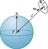
This is sometimes called the rule of five.
The notion of irradiance appears in many research papers about rendering, and it’s often given the letter E. Except for brief mention in our discussion of radiosity in Chapter 31, we’ll have no further use for irradiance, and we will use the letter E primarily to denote the eyepoint (or camera) in a rendering algorithm.
26.7.5. Radiant Exitance
The corresponding measure of light leaving a surface in all possible directions is called spectral radiant exitance; the only difference is the direction of the vector ωo appearing in L:
Once again, we’re defining this for reflective-only surfaces. And we can again extend this to be defined at any point in space: As long as we provide an additional argument indicating a surface normal, and by integrating over all wavelengths, we get the radiant exitance.
26.7.6. Radiant Power or Radiant Flux
The radiant power or radiant flux Φ arriving at a surface M (whether it’s an actual surface in the scene or some virtual surface like “the surface of a sphere of radius 1 m surrounding this light source”) is computed by integrating yet again. Since power is measured in joules per second, we must integrate over a region to remove the m2 from the units:
The units of (spectral) power are J s–1 nm–1; those of power (arrived at by integrating out wavelength) are J/ sec, that is, W.
The meaning of “power” is only well defined when the surface M over which we are integrating is specified (along with the time and the wavelength).
For an imaginary surface in space, like the sphere surrounding the light source above, the power arriving at one side of the surface and the power leaving the opposite side are the same; for an actual surface in the scene, the power arriving at one side of a surface may be large, but for opaque surfaces, no power leaves the other side, although usually a lot is reflected.
To define radiant flux for a surface that both reflects and transmits, we need to extend the domain of integration to all of S2, and place absolute values on the dot product:
What is the domain of the “Power” function? Certainly time and wavelength are still arguments, but what about the surface at which the power is arriving? One possible answer is that M, the thing over which the integral is computed, can be any measurable subset of any surface in 3-space. (There’s no standard name for the set of all such subsets). Most books simply ignore the question, and speak of the “radiant flux Φ,” whose domain is ignored. We’ll return to this briefly in Section 26.9.
26.8. Other Measurements
All radiometric quantities can be expressed as integrals of L: For the spectral radiant intensity, which we mentioned briefly above, with units of watts per steradian, you integrate out area and wavelength. For the nonspectral version, you also integrate out wavelength. Radiosity is a name sometimes used in graphics for a nonspectral radiant exitance; its units are watts per square meter (one integrates out wavelength and directions).
Terms like these (and like “irradiance” and “radiant exitance”) are useful when we try to describe the flow of light energy in a scene with an approximation in which we aggregate light in various ways. For example, if our scene consists entirely of diffuse reflectors (e.g., items painted with a coat of latex paint), then it makes sense to do computations that ignore the direction in which light is radiated, and simply compute the total light energy radiated from a surface. In the same way, we often aggregate light into three wavelength groups, which we call “red,” “green,” and “blue,” so that instead of computing the light transport individually for every possible wavelength λ, we simply compute it for three aggregates. This results in approximations of the correct results, but in many cases the approximations can be very good. Indeed, it’s often worth writing the light energy leaving a surface as a sum of terms, each of which can be studied by a suitable algorithm; in some of these algorithms summary representations of the light may be appropriate, whereas in others the highly detailed representation provided by the radiance field L is more appropriate.
There are also other quantities that describe aggregate properties of light in terms that are relevant to human perception; these lie in the domain of photometry and are discussed in Section 28.4.1.
Finally, there is a term that can cause considerable difficulty: intensity. Intensity occurs frequently in early graphics papers, but its meaning is rarely given precisely. It’s probably best to read these papers with a modern eye and regard “intensity” as a proxy for “radiance,” although there may be a cosine factor or two missing in any particular discussion. When we use the word “intensity,” it’s strictly informal, as in the sentence “When we increase the intensity of the lamp, the scene brightens.”
26.9. The Derivative Approach
An alternative approach to defining radiometric terms is to take the radiant flux Φ as a starting point, and to derive all other quantities from it through a kind of “differentiation.” For instance, we can look at a point P of some surface, and a region R on the surface with P ![]() R, and consider the light arriving at R from all possible directions, and the resultant power arriving at R, which we call ΔΦ. By dividing this power ΔΦ by the area of R, ΔA, we get a power-per-area measurement,
R, and consider the light arriving at R from all possible directions, and the resultant power arriving at R, which we call ΔΦ. By dividing this power ΔΦ by the area of R, ΔA, we get a power-per-area measurement,
If we imagine repeating this process for various regions R, each with a smaller and smaller area, but still containing the point P, we get a sequence of power-per-area measurements. The argument is then that these measurements have a limit, as the area of the region R goes to zero, and we call this limit
the irradiance at P.
Before proceeding further with this approach, we ask that you carefully review the definition of the derivative. Typically when we write df/dx, we require that f be a function of a variable x, and that ![]() have a limit as h
have a limit as h ![]() 0; this limit is called the derivative. In the formulation above, there’s no “variable” A, and Φ is certainly not a function of A. We can repair this problem by saying, “Let f (r) be the power arriving at a disk of radius r about P in the surface; the area of that disk is πr2, and we can define g(r) = f (r)/(πr2), which represents the power arriving at the disk, per area. We then define dΦ/dA(P) to be g′ (0).” But one then must ask, “Would the result have been the same if I’d used a family of shrinking squares rather than disks? What about other shapes? And is g obviously differentiable?” And for each new concept defined by a “derivative” like this one, one has to reconsider the corresponding questions. The integral formulation we have pursued makes one single assumption—the existence of an integrable spectral radiance function L—and everything else follows from that.
0; this limit is called the derivative. In the formulation above, there’s no “variable” A, and Φ is certainly not a function of A. We can repair this problem by saying, “Let f (r) be the power arriving at a disk of radius r about P in the surface; the area of that disk is πr2, and we can define g(r) = f (r)/(πr2), which represents the power arriving at the disk, per area. We then define dΦ/dA(P) to be g′ (0).” But one then must ask, “Would the result have been the same if I’d used a family of shrinking squares rather than disks? What about other shapes? And is g obviously differentiable?” And for each new concept defined by a “derivative” like this one, one has to reconsider the corresponding questions. The integral formulation we have pursued makes one single assumption—the existence of an integrable spectral radiance function L—and everything else follows from that.
Having made this critique of the “derivative” formulation, we should also mention its advantages. One of these is that when you write
you know that if you want to compute the power, Φ, you’ll need to compute an integral,
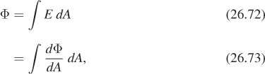
with the obvious notion that “the dAs cancel.” In our experience, the presence of various cosines makes this sort of computation fraught with peril. Our students routinely draw false conclusions by being insufficiently precise about what they mean in such derivations. On the other hand, once you have some experience with this notation, and have gotten past the usual mistakes, it’s a great convenience.
To continue with the standard derivative description, the radiant exitance is also defined as a derivative of power with respect to area,
where this time Φ means the power leaving the surface rather than arriving there.
The radiant intensity (a term we haven’t previously defined, and will not mention again) is the derivative of flux with respect to solid angle,
and radiance is the “radiant flux per unit solid angle per unit projected area” [Jen01],
where θ is the angle between ω and the surface normal. This description of L is then inverted to write
The experienced reader knows how to read this: “The total power arriving at a region A with surface normal n, along rays in the solid angle Ω, is given by Equation 26.77.”
26.10. Reflectance
How can we model reflectance? We’d like to somehow capture the idea that light striking a bit of surface from some distant point may scatter in many different directions, and that light from many different directions may therefore contribute to the light leaving in some particular direction. The great insight is to realize that the process is additive: If we can measure how light from each single direction is scattered, we’ll know how light from a whole collection of directions is scattered as well.
A gonioreflectometer is a device used to measure reflectance; in the most basic design, it consists of a tiny spotlight mounted so that it can move about on a spherical shell, and a tiny sensor that can also move about on the shell (see Figure 26.31). (More modern designs, like the one shown in Figure 26.32, rely on moving the sample stage in more directions, rather than both the source and detector.)
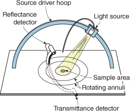
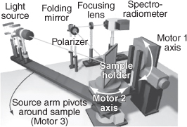
Figure 26.32: A modern gonioreflectometry system. (Courtesy of Steve Westin, “Automated three-axis gonioreflectometer for computer graphics applications” by Westin, Foo, Li, and Torrance, from Advanced Characterization Techniques for Optics, Semiconductors, and Nanotechnologies II, Proc. SPIE 5878, August 2005).
The spotlight illuminates a sample placed at the center of the sphere, and the sensor detects the amount of light bouncing off the sample. (The region around the sample, and the inside of the sphere, are coated with a light-absorbing material like lampblack.) When the light source is shining on the sample at a grazing angle, the recorded reflection values are quite small (partly because so much of the illumination hits the black paint around the sample rather than the sample itself). One can imagine raising the intensity of the spotlight so that the total energy falling on the sample is constant, independent of the spotlight location; to do so, we’d have to multiply the basic intensity by ![]() , where φ is the colatitude of the spotlight. Because this would require some difficult engineering, we instead simply multiply the sensor reading by that value.
, where φ is the colatitude of the spotlight. Because this would require some difficult engineering, we instead simply multiply the sensor reading by that value.
So, what does the gonioreflectometer measure? Assuming for the moment that the radius of the sphere is so large, and the spotlight, sensor, and sample are so small, that areas and solid angles can be treated as infinitesimal, it measures
where
• Ω is the solid angle subtended by the light source at the sample, and we’ve written m(Ω) to indicate its measure
• ωi and ωo are respectively the directions from the sample to the source and to the sensor
You can purchase a radiance meter; the light meter used by photographers is a crude version. The computation done to get readings from the gonioreflectomer, is this: first measure the radiance, L1, arriving from the light source. Measure the area, A, of the light source, and its distance, r, from the sample. The solid angle it subtends is then A/r2. Now for each (ω, ω′) pair, place the light source so that light arrives in direction –ω, and the radiance sensor so that it detects the radiance from the sample in direction ω. Call this radiance value L2. Then the “reading” from the gonioreflectometer is ![]() ). In practice, it’s best to measure
). In practice, it’s best to measure ![]() , the radiance from the sample when the illuminator is off, and L
, the radiance from the sample when the illuminator is off, and L![]() , the radiance with the illuminator on, and then compute
, the radiance with the illuminator on, and then compute ![]() ; this prevents the too-high readings for grazing angles that can arise when stray light enters the device, or when there’s some offset in the calibration of the radiance meter, so that even total darkness registers as having some positive radiance.
; this prevents the too-high readings for grazing angles that can arise when stray light enters the device, or when there’s some offset in the calibration of the radiance meter, so that even total darkness registers as having some positive radiance.
We call fr the (spectral) bidirectional reflectance distribution function, or BRDF. Note that fr has units of sr–1. Because the gonioreflectometer light source is constant (i.e., the radiance leaving it is constant), the value defining fr is independent of time. One can extend the definition of fr to directions ωi and ωo “on the wrong side” of the surface by defining it to be zero there. The domain of fr is then
where M is the collection of all surfaces in the world. Note that in the definition of fr(P, ωi, ωo, λ), the vector ωi is a unit vector pointing toward the incoming light, so the incoming light is traveling in direction –ωi.
With this definition of fr, the correct form for relating the outgoing radiance Lr from a surface to the incoming radiance Li is
because the cosine of the colatitude of the incoming direction is just the negative dot product of that direction vector and the outward surface normal. This is the reflectance equation, the central part of a more general rendering equation [Kaj86, ICG86, NN85], to which we’ll return in Chapter 29.
Because of the cosine factor, some books describe reflectance as the ratio of outgoing radiance to incoming irradiance. We’ve instead defined it directly in terms of Li for clarity.
The BRDF generally has an important symmetry called Helmholtz reciprocity:
This tells us, for example, that we need not place the light source and sensor at every possible pair of positions when we measure the BRDF with a gonioreflectometer; we can skip half of the positions.
But the Helmholtz reciprocity law also tells us that not just any function can be the BRDF of a material. In fact, there are further restrictions. For instance, if a certain amount of power arrives at a surface and is reflected, the amount of power leaving the surface must be no more than the amount that arrived, because of energy conservation. This places restrictions on various integrals of the BRDF.
Helmholtz reciprocity holds for a great many materials; indeed, there have been several purported proofs of it. Those proofs are thrown into doubt by the existence of materials that have been measured and shown to not satisfy the “law.” Veach [Vea97] discusses the hypotheses necessary for reciprocity to hold.
26.10.1. Related Terms
A thin sheet of colored vinyl may both reflect light and transmit it; in such a case, one can build a gonioreflectometer to measure the transmitted light instead of the reflected light; the portion of the function fr that we’d defined as zero for purely reflective surfaces becomes nonzero in this case, and the “reflectance” portion of the function is set to zero. The resultant function is called the bidirectional transmittance distribution function, or BTDF.
The sum of these two is called the bidirectional scattering distribution function, or BSDF, which we’ll denote fs.
When a ray of light meets a surface at a point P, we’ve been assuming that it is reflected (or transmitted) and again leaves from the point P. In many interesting materials, including human skin, hair, many forms of wood, and tree leaves, light actually enters the material, reflects multiple times under the surface, and is reemitted from some point near P (see Figure 26.33). This scattering is characterized by a bidirectional surface scattering reflectance distribution function, or BSSRDF, which has, as arguments, the point P, the direction of the arriving light ωi, the point Q from which the light exits, and the direction ωo in which it exits. Fortunately, for many surfaces the simpler BSDF suffices. Rendering materials using the BSSRDF, however, can produce some spectacular results [JMLH01] (see Figure 26.34).
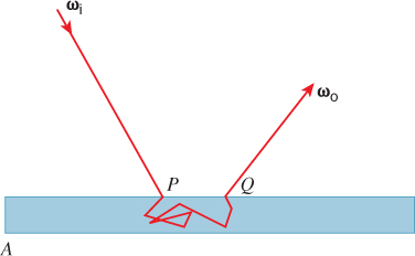
Figure 26.33: Subsurface scattering. To describe the scattering of light that arrives in direction –ωi at a point P of a surface that’s not a pure reflector, but rather allows multiple subsurface bounces before the light is emitted, requires a description of the emitted light at every nearby point Q in every outgoing direction ωo.

Figure 26.34: Subsurface scattering lets light pass through the marble and skin in these images. (Courtesy of Stephen Marschner, ©2001 ACM, Inc. Reprinted by permission.)
26.10.2. Mirrors, Glass, Reciprocity, and the BRDF
Imagine trying to measure the BRDF for a perfect mirror using a gonioreflectometer. The sensor computes the incoming radiance by measuring the arriving power and dividing by the sensor area, which implicitly makes the assumption that the radiance along all rays from the sample to the sensor is approximately constant. But if the source is so tiny that its reflected rays all lie well within the sensor area, this assumption is invalid: For much of the sensor, no light is arriving at all. So a gonioreflectometer for measuring the BRDF of a mirror must have a sensor whose size is adjustable so that the whole sensor area is saturated with light. Of course, because mirror reflection is so “concentrated” (the rays of light don’t spread out at all after reflection), it makes sense to try to measure the BRDF with a very tiny light source, perhaps a source with an adjustable iris. As we shut down the iris on the source, we’ll have to make the sensor area smaller to compensate. The one thing we know is that the radiance of a ray from the source to the sample is the same as the radiance from the sample to the sensor, because the material is a perfect mirror. Now consider our definition for the BRDF:
Suppose we first perform the measurement with a source at φ = 0 whose solid angle, measured from the sample, is 0.01 sr. The two radiances in the formula are the same, so they cancel, and the BRDF measurement is 100 sr–1.
Now suppose that we close down the iris on the light source so that it subtends a solid angle of 0.005 sr. We’ll have to shrink the sensor as well to get a valid radiance measurement, but when we do so we’ll again find that the received radiance is the same as the emitted radiance. The BRDF measurement will be 200 sr–1. As we continue closing the iris, the measurements will increase without bound. The conclusion is that for a perfect mirror, the BRDF is infinite. To be more precise: If the reflection of ωi is ωo, and the surface being measured is a mirror, then fr(P, ωi, ωo, λ) is infinite.
It doesn’t actually make sense to say that a function takes on the value “infinity,” but there is a mathematical theory of a different class of objects, called distributions, which can take on infinite values. The name “bidirectional reflectance distribution function” reflects this. One difficulty with this notion of infinite values arises when we consider an imperfect mirror, one that reflects only half the arriving light, and absorbs the rest. If we carry out the preceding analysis for such a mirror, we find that its BRDF also takes on an infinite value for mirror reflection, but we have the sense that it’s a “different infinity” that’s only half as big. We’ll circumvent these problems by splitting any BRDF into two parts: a “diffuse” part and an “impulse” part, where the latter is a representation of things like mirror reflection and Snell’s law refraction.
If we ignore, for a moment, the problem of the infinite values, we can still look at the formula for fr and consider the cosine that appears there. What happens when we swap the roles of ωi and ωo for the perfect mirror? Since the incoming and outgoing radiances are equal, the only possible change is in the cosine. But for a mirror reflection, the incoming and outgoing angles are equal; this means that to the degree that fr makes any sense at all, it seems to satisfy Helmholtz reciprocity.
On the other hand, when it comes to measuring fs for a material like glass, the transmissive part of the computation involves two different angles, determined by Snell’s law. It’s evident that in this case, even if we can make sense of the infinite value of fs, it will not satisfy the reciprocity law.
26.10.3. Writing L in Different Ways
The function L is defined on R × R3 × S2 × R+. Thus, it makes sense to write expressions like L(t, P, ω, λ), where ω ![]() S2 and P
S2 and P ![]() R3; it makes equally good sense to write L(t, x, y, z, ω, λ), where x, y, and z are real numbers. In a computer program, of course, assuming that “point in 3-space” is a class of objects, we’d have to use an overloaded function, with arguments of type
R3; it makes equally good sense to write L(t, x, y, z, ω, λ), where x, y, and z are real numbers. In a computer program, of course, assuming that “point in 3-space” is a class of objects, we’d have to use an overloaded function, with arguments of type real * point3 * spherepoint * real or real * real * real * real * spherepoint * real, but the distinction between the two would be so tiny that it wouldn’t matter.
But the spherepoint class is trickier. One can choose to characterize each point on the unit sphere by its (θ, φ) coordinates, but those two numbers are not the same thing as the point on the sphere. One could also represent the point by its (x, y, z) coordinates, although in a practical sense it’s very hard to find computer-based real numbers satisfying x2 + y2 + z2 = 1 exactly. In engineering and physics it’s common to gloss over these difficulties, and, for a function U defined on S2, write things like
where
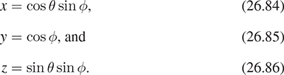
Unfortunately, this sort of overloading, although it can be used in computer programs sometimes, makes little sense in mathematics. The symbol U can mean only one thing.
For this reason, we’ll carefully reserve the symbol L to denote the function whose domain is R × R3 × S2 × R+; when we need one of the closely related functions (e.g., defined in terms of polar angles in Chapter 27), we’ll give it a new name to distinguish it from the original. Later when we discuss rendering algorithms, we’ll be making a steady-state assumption (that L(t, ...) is independent of the parameter t), and the wavelength parameter λ will never enter into any formulas in any significant way, so we’ll write L(P, ω) instead of L(t, P, ω, λ).
26.11. Discussion and Further Reading
We’ve described how light energy is measured, and given some details of the microscopic characteristics of light and their relationship to the characteristics of the matter with which light interacts, but proper treatment of these belongs in the realm of physics. A superb first reference is Crawford’s book on waves [Cra68]. One should also understand some electromagnetic theory [Pur11]. Anyone who studies graphics will also benefit from even a partial reading of Newton’s Opticks [New 18]. It teaches not only the ideas of optics, but how a brilliant observer and experimenter works. For the application of these ideas in practical algorithms, see the book by Pharr and Humphreys [PH10].
We’ve discussed the radiometric terms used in measuring light, but there are also photometric terms, which attempt to capture the human perception of light. In particular, light of different wavelengths can be perceived as equally bright, and so by summing up the radiance at many different wavelengths, each multiplied by a factor ![]() (λ) representing the perceived brightness of a certain amount of light energy at wavelength λ, you can get a single number (called luminance) that represents total brightness. The function
(λ) representing the perceived brightness of a certain amount of light energy at wavelength λ, you can get a single number (called luminance) that represents total brightness. The function ![]() is called the luminous efficiency; it also is used in the CIE color system, which we discuss in Chapter 28. Luminance is measured in lumens. Such a single number for brightness of a light makes sense in contexts where most light is broad-spectrum, and most reflectors reflect light across much of the spectrum. But because light energy and reflectivity are spectral quantities, it’s possible to have a light of high luminance (e.g., a bright red laser) and a surface with high reflectivity (where this reflectivity is an average over all wavelengths of the spectral reflectivity), and yet have the reflected light be low luminance, if the surface, for example, happens to absorb rather than reflect light at the wavelength of the laser. Because of this, such photometric terms see little use in graphics, but they are of considerable importance in illumination engineering.
is called the luminous efficiency; it also is used in the CIE color system, which we discuss in Chapter 28. Luminance is measured in lumens. Such a single number for brightness of a light makes sense in contexts where most light is broad-spectrum, and most reflectors reflect light across much of the spectrum. But because light energy and reflectivity are spectral quantities, it’s possible to have a light of high luminance (e.g., a bright red laser) and a surface with high reflectivity (where this reflectivity is an average over all wavelengths of the spectral reflectivity), and yet have the reflected light be low luminance, if the surface, for example, happens to absorb rather than reflect light at the wavelength of the laser. Because of this, such photometric terms see little use in graphics, but they are of considerable importance in illumination engineering.
26.12. Exercises
Exercise 26.1: We claimed in the chapter that the horizontal projection P to the unit sphere from the vertical cylinder enclosing it was an area-preserving map. Compute the derivative of this map at a point (x, y,0) of the cylinder, and verify that it is area-preserving. Why is it sufficient to carry out this computation at a point where z = 0?
Exercise 26.2: We computed the solid angle subtended by a spherical cap of radius r < π on the unit sphere as 2π(1 – cos(r)).
(a) What is the solid angle subtended by a spherical cap of radius r on a sphere of radius R?
(b) What is the actual area of a spherical cap of radius r on a sphere of radius R? You should be able to do this problem almost by inspection, without any integrals at all.
![]() Exercise 26.3: We computed the radiance emitted from each point of a spherical uniform source of radius r and total power Φ in each outward direction ω as
Exercise 26.3: We computed the radiance emitted from each point of a spherical uniform source of radius r and total power Φ in each outward direction ω as ![]() . Now consider some distant point P, lying on a surface that faces the center C of the spherical source, and that the distance from C to P is R >> r. We can compute the irradiance at P by computing the solid angle subtended by the spherical source, and the radiance arriving at P along each direction of that solid angle, etc.
. Now consider some distant point P, lying on a surface that faces the center C of the spherical source, and that the distance from C to P is R >> r. We can compute the irradiance at P by computing the solid angle subtended by the spherical source, and the radiance arriving at P along each direction of that solid angle, etc.
(a) Do this computation to determine the irradiance at P.
(b) Now suppose that the total power Φ remains constant, while the radius r of the source shrinks. What is the limit of the expression you found in part (a) as r ![]() 0?
0?
Exercise 26.4: It would be nice to imagine a “beam” of light arriving at a point P of a surface in direction ωi, and being reflected out in many directions; we could then look at how much light goes in each direction and talk about the “scattering” from the surface. The problem is that light arriving at a single point cannot carry any energy, and light arriving in a single direction cannot carry any energy. Instead, we can imagine light arriving in directions η with |η – ωi| ≤ (i.e., directions very nearly parallel to ωi), and arriving at points ||Q with Q – P|| < r, for some small r, with constant radiance ![]() . In this problem, we’ll examine the irradiance due to this “beam.” If the BRDF is continuous as a function of position and incoming direction, then the outgoing radiance in direction ωo will vary smoothly as a function of r and
. In this problem, we’ll examine the irradiance due to this “beam.” If the BRDF is continuous as a function of position and incoming direction, then the outgoing radiance in direction ωo will vary smoothly as a function of r and ![]() .
.
(a) What’s the solid angle of the incoming rays as a function of? What’s a simplified expression for small ![]() ?
?
(b) How should we adjust the radiance ![]() along incoming rays, as we reduce r and toward zero, to make certain that the incoming power is constant? When we adjust the incoming radiance in this way, and take a limit, we can speak of a beam of light in direction ωi having a certain irradiance; the resultant radiance in direction ωo can then be measured (theoretically). The ratio
along incoming rays, as we reduce r and toward zero, to make certain that the incoming power is constant? When we adjust the incoming radiance in this way, and take a limit, we can speak of a beam of light in direction ωi having a certain irradiance; the resultant radiance in direction ωo can then be measured (theoretically). The ratio
has a limit as and r go to zero because of the form of ![]() , and the limit is exactly the BRDF; this is the justification for defining the BRDF as “the ratio of the outgoing radiance in direction ωo to the incoming radiance of a beam in direction ωi.” Therefore, the integral of the BRDF, over all outgoing directions, multiplied by ωo · n, tells how much of the power arriving in the beam gets reflected in any direction at all, and is therefore called the directional hemispherical reflectance.
, and the limit is exactly the BRDF; this is the justification for defining the BRDF as “the ratio of the outgoing radiance in direction ωo to the incoming radiance of a beam in direction ωi.” Therefore, the integral of the BRDF, over all outgoing directions, multiplied by ωo · n, tells how much of the power arriving in the beam gets reflected in any direction at all, and is therefore called the directional hemispherical reflectance.
Exercise 26.5: Latex wall paint is designed to be Lambertian, that is, it’s designed so that when illuminated by light from any direction, it has the same apparent brightness regardless of the direction from which it’s viewed (i.e., the radiance along every outgoing ray is the same). Furthermore, the outgoing radiance should be independent of the incoming direction of the illumination, so long as the power arriving at a fixed region of the painted surface is constant. Good latex paint very nearly achieves this goal, although at grazing angles the reflectance varies from the ideal. If it were such an ideal reflector, what would its BRDF look like?
Exercise 26.6: A planar surface S sits in a room that’s bathed in light so that the radiance along every ray arriving at S is the same constant, 10 watts per steradian per square meter. What’s the irradiance at a point P of the surface?
Exercise 26.7: Two incandescent bulbs emit the same total power in the visible spectrum; one has a filament at 4000 K, the other at 6500 K. Because of the Stefan-Boltzmann law, the second filament must be much smaller than the first. Which one emits more power in the invisible portion of the spectrum?
Exercise 26.8: A student is given data captured from a digital camera; the scene viewed by the camera is a spherical frosted incandescent lamp that emits 1.2 W of power in the visible range. The lamp has a radius of 0.0175 m. The camera shutter speed has been adjusted so that the sensor is neither saturated nor starved; indeed, the values in the image are near the center of the camera’s pixel-value range, and can be assumed to be proportional to radiance. The value observed for pixels that lie in the lamp is 4000 (on a scale from 0 to 8191). The student wants to know the constant of proportionality between the radiance of arriving light and the sensor value. The student says, “The lamp is supposed to emit uniformly because of its frosting, so except for really tangential angles, we can figure that the radiance of all outgoing rays is constant. The area of the lamp is 4πr2 ≈ 0.000 962 m2; the hemisphere over which the light is radiated has solid angle measure approximately 6.28 sr, so the radiance, by division, is the power divided by the angle and the area, giving L ≈ 1.2 W/(0.000 962 m2 * 6.28 sr) ≈ 0.006 W/m2sr. So to get the radiance L from the sensor value, we multiply by ![]() Critique the student’s approach, and give the correct answer.
Critique the student’s approach, and give the correct answer.
![]() Exercise 26.9: We said that “A ‘disk’ consisting of all points on the unit sphere whose spherical distance from a point P is less than r (where r < π) has solid angle measure 2π(1 – cos(r)).” But you’d expect, for small r, that the solid angle would contain an r2 factor, because the formula for the area of a disk in the plane contains an r2 factor. Reconcile the two by recalling the Taylor series for cos(r) at r = 0.
Exercise 26.9: We said that “A ‘disk’ consisting of all points on the unit sphere whose spherical distance from a point P is less than r (where r < π) has solid angle measure 2π(1 – cos(r)).” But you’d expect, for small r, that the solid angle would contain an r2 factor, because the formula for the area of a disk in the plane contains an r2 factor. Reconcile the two by recalling the Taylor series for cos(r) at r = 0.
Exercise 26.10: Consider a disk of radius s in the plane, centered at the origin, and the point P = (0, 0, –h) that’s distance h below the disk. Assume that the disk is a Lambertian emitter, emitting radiance L in every direction from every point, and is the only surface in the scene.
(a) Write out an integral for the irradiance at P.
(b) Evaluate the integral. Switching to polar coordinates on the plane will help.
(c) Show that if h < s/10, then the irradiance at P is essentially the same as it would be if the disk covered the entire plane (i.e., if s were very large). Thus, for small values of h, the irradiance is nearly constant.
(d) Show that for h > 5s, the irradiance is within 5% of πL(s/h)2.
Exercise 26.11: Show that any plane wave E traveling along the x-axis as in Equation 26.6 can be expressed as the sum of two plane waves, E| and E°, the first being linearly polarized and the second being circularly polarized. Hints: The axis of the linearly polarized wave will be [0 Ay Az]T; the magnitude of the circularly polarized wave will be ![]() .
.
Exercise 26.12: Suppose that in Figure 26.11, we draw a circle of radius r about the refraction point. On the line tangent to the top of this circle, we place equispaced points, and from each point draw a ray toward the refraction point. These rays refract with different angles into the lower material. Each refracted ray meets a horizontal line tangent to the bottom of the circle.
(a) Draw a figure depicting this situation.
(b) Show that the points of intersection on the bottom line are also equispaced.
(c) What is the ratio of the bottom-line spacing to the top-line spacing?
Exercise 26.13: Use Planck’s formula for blackbody radiation R(f, T) in terms of frequency to approximate the location of the power peak in R(f, T) as a function of T (i.e., for fixed T, find the f that maximizes power). Show that this is roughly linear in T. (This is known as Wien’s displacement law.) To do so, fix T, and define a variable u = f /T, and write R(f, T) as a function ![]() where D(u) = e(h/k)u – 1, which depends only on the single variable u. Under what condition on u is S(u) a maximum? (You may assume that e(h/k)u >> 1.)
where D(u) = e(h/k)u – 1, which depends only on the single variable u. Under what condition on u is S(u) a maximum? (You may assume that e(h/k)u >> 1.)
For T near 10,000°K (roughly the temperature of the surface of the sun), the peak is at about frequency 5 × 10¹⁴ Hz, which is just about in the middle of the range of visible light (roughly 4 × 10¹⁴ Hz to 7 × 10¹⁴ Hz); this means that the human visual system is most sensitive to the energy that’s most common (sun-light).