
1.3 Almost-Cyclostationary Processes
Many processes encountered in telecommunications, radar, mechanics, radio astronomy, biology, atmospheric science, and econometrics, are generated by underlying periodic phenomena. These processes, even if not periodic, give rise to random data whose statistical functions vary periodically with time and are called cyclostationary processes. In this section, the properties of cyclostationary, or more generally, of almost-cyclostationary processes are briefly reviewed. For extensive treatments, see (Gardner 1985, Chapter 12, 1987d), (Gardner et al. 2006), (Giannakis 1998), (Hurd and Miamee 2007).
1.3.1 Second-Order Wide-Sense Statistical Characterization
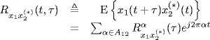
The (finite-power) process x(t) is said to be second-order cyclostationary in the wide sense or periodically correlated with period T0 if its first-and second-order moments are periodic functions of time with period T0. More generally, first-and second-order moments can be almost-periodic functions of time (in one of the senses considered in Section 1.2) and the process is said to be second-order almost-cyclostationary (ACS) in the wide sense or almost-periodically correlated (Gardner 1985, Chapter 12, 1987d). In such a case, its (conjugate) autocorrelation function (1.6) under mild regularity conditions can be expressed by the (generalized) Fourier series expansion
where subscript ![]() , A is the countable set (depending on (*)) of possibly incommensurate cycle frequencies α, and the Fourier coefficients
, A is the countable set (depending on (*)) of possibly incommensurate cycle frequencies α, and the Fourier coefficients
![]()
referred to as the (conjugate) cyclic autocorrelation functions, are complex-valued functions whose magnitude and phase represent the amplitude and phase of the finite-strength additive sinewave component at frequency α contained in ![]() . Thus,
. Thus, ![]() if α
if α ![]() A and
A and ![]() if
if ![]() . Cyclostationary processes are obtained as a special case when
. Cyclostationary processes are obtained as a special case when ![]() . WSS processes are a further specialization when A contains the only element α = 0.
. WSS processes are a further specialization when A contains the only element α = 0.
The function (1.87) is the time-lag (conjugate) autocorrelation function of ACS processes. By substituting t = t2 and τ = t1 − t2 into (1.87), one obtains the time-time (conjugate) autocorrelation function of ACS processes
For a zero-mean process x(t) with finite or practically finite memory the result is that ![]() as |τ|→ ∞. In contrast, if the process has non-zero almost-periodic expectation E{x(t)}, then some
as |τ|→ ∞. In contrast, if the process has non-zero almost-periodic expectation E{x(t)}, then some ![]() contain additive sinusoidal functions of τ which arise from products of finite-strength sinusoidal terms contained in E{x(t)} (Gardner and Spooner 1994). ACS signals in communications are zero mean unless pilot tones are present for synchronization purposes. In mechanical applications, ACS signals generally have an almost-periodic expected value (Antoni 2009). For the following, let us assume that
contain additive sinusoidal functions of τ which arise from products of finite-strength sinusoidal terms contained in E{x(t)} (Gardner and Spooner 1994). ACS signals in communications are zero mean unless pilot tones are present for synchronization purposes. In mechanical applications, ACS signals generally have an almost-periodic expected value (Antoni 2009). For the following, let us assume that
Such an assumption is verified by finite-memory or practically finite-memory signals. From (1.89) it follows that ![]() for p ≥ 1 and
for p ≥ 1 and ![]() for p ≥ 1.
for p ≥ 1.
By Fourier transforming with respect to τ both sides of (1.87) we obtain the almost-periodically time-variant spectrum
where
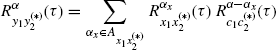
is the (conjugate) cyclic spectrum which can be expressed as
(1.92) ![]()
where the order of the two limits cannot be reversed and
is the short-time Fourier transform (STFT) of x(t). Therefore, the (conjugate) cyclic spectrum is also called the (conjugate) spectral correlation function and (1.91) is the Gardner Relation (Gardner 1985) (also called Cyclic Wiener-Khinchin Relation). Under assumption (1.89) the Fourier transform ![]() exists in the ordinary sense. Accordingly with (1.90), the Wigner-Ville spectrum (1.20a) of an ACS signal is an almost-periodic function of t′ with frequencies α
exists in the ordinary sense. Accordingly with (1.90), the Wigner-Ville spectrum (1.20a) of an ACS signal is an almost-periodic function of t′ with frequencies α ![]() A and Fourier-series coefficients
A and Fourier-series coefficients ![]() .
.
From (1.8), (1.14b), and (1.87), in the case of ACS processes, one obtains the following Loève bifrequency spectrum
That is, ACS processes have Loève bifrequency spectrum with spectral masses concentrated on a countable set of lines with slope ±1. Equivalently, ACS processes have distinct spectral components that are correlated only if the spectral separation belongs to a countable set which is the set A of the cycle frequencies.
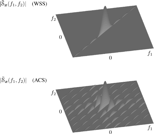
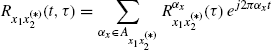
In Figures 1.3 and 1.4, the magnitude of the cyclic autocorrelation as a function of α and τ and the magnitude of the bifrequency spectral correlation density ![]() (obtained by replacing in (1.23) and (1.94) Dirac deltas with Kronecker ones) as a function of f1 and f2 are reported for a WSS and an ACS signal. The ACS signal is a cyclostationary PAM with a rectangular pulse q(t). The considered WSS signal has the same autocorrelation function and power spectrum of the PAM signal. The WSS signal has a nonzero cyclic autocorrelation function only for α = 0 (Figure 1.3 (top)). Equivalently, the bifrequency spectral correlation density in nonzero is only on the main diagonal of the bifrequency plane (Figure 1.4 (top)). In contrast, the ACS signal has a nonzero cyclic autocorrelation function in correspondence of the cycle frequencies which are multiples of a fundamental one (Figure 1.3 (bottom)). Equivalently, the bifrequency spectral correlation density is nonzero on lines which are parallel to the main diagonal so that spectral components which are correlated are separated by quantities equal to the cycle frequencies (Figure 1.4 (bottom)).
(obtained by replacing in (1.23) and (1.94) Dirac deltas with Kronecker ones) as a function of f1 and f2 are reported for a WSS and an ACS signal. The ACS signal is a cyclostationary PAM with a rectangular pulse q(t). The considered WSS signal has the same autocorrelation function and power spectrum of the PAM signal. The WSS signal has a nonzero cyclic autocorrelation function only for α = 0 (Figure 1.3 (top)). Equivalently, the bifrequency spectral correlation density in nonzero is only on the main diagonal of the bifrequency plane (Figure 1.4 (top)). In contrast, the ACS signal has a nonzero cyclic autocorrelation function in correspondence of the cycle frequencies which are multiples of a fundamental one (Figure 1.3 (bottom)). Equivalently, the bifrequency spectral correlation density is nonzero on lines which are parallel to the main diagonal so that spectral components which are correlated are separated by quantities equal to the cycle frequencies (Figure 1.4 (bottom)).
Figure 1.3 Magnitude of the cyclic autocorrelation function of a signal x(t) as functions of α and τ. Top: WSS signal. Bottom: ACS signal
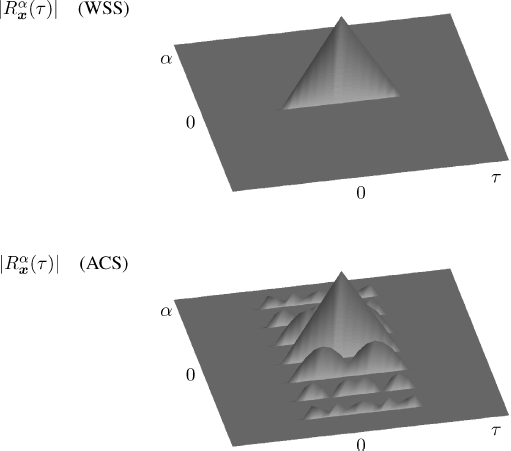
Figure 1.4 Magnitude of the bifrequency spectral correlation density of a signal x(t) as functions of f1 and f2. Top: WSS signal. Bottom: ACS signal
1.3.2 Jointly ACS Signals
Let ![]() , be two complex-valued almost-cyclostationary (ACS) continuous-time processes with second-order (conjugate) cross-correlation function
, be two complex-valued almost-cyclostationary (ACS) continuous-time processes with second-order (conjugate) cross-correlation function
where
(1.96) ![]()
is the (conjugate) cyclic cross-correlation function of x1 and x2 at (conjugate) cycle frequency α and
is a countable set. If the set A12 contains at least one nonzero element, then the time series x1(t) and x2(t) are said to be jointly ACS. Note that, in general, the set A12 depends on whether (*) is a conjugation or not and can be different from the sets A11 and A22 (both defined according to (1.97)).
The (conjugate) cyclic cross-spectrum of x1 and x2 at (conjugate) cycle frequency α is defined as
and is related to the (conjugate) cyclic cross-correlation function by the Gardner relation
(1.99) ![]()
In (1.98), ![]() is the STFT of
is the STFT of ![]() defined according to (1.93).
defined according to (1.93).
In the case of distinct processes (or processes denoted as distinct), the use of optional conjugation can be avoided without a lack of generality. In fact, if ![]() , then
, then ![]()
![]() . However, the following results are useful for future reference. Let
. However, the following results are useful for future reference. Let ![]() , where superscript (*)i denotes ith optional complex conjugation.
, where superscript (*)i denotes ith optional complex conjugation.
If
then
where (−)i is an optional minus sign linked to (*)i.
In fact, by making the variable change ![]() ,
, ![]() into (1.100) the result is that
into (1.100) the result is that
(1.102) ![]()
and in the sense of distributions we formally have
(1.103) 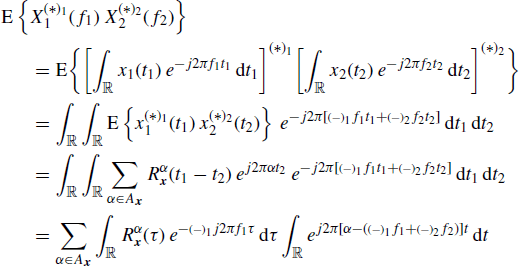
from which (1.101) follows since
(1.104) 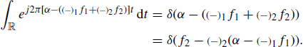
By specializing (1.100) and (1.101) we have
(1.105) ![]()
(1.106) ![]()
1.3.3 LAPTV Systems
Linear almost-periodically time-varying (LAPTV) systems have an impulse-response function that can be expressed by the (generalized) Fourier series expansion
or, equivalently,
(1.108) ![]()
where J is a countable set of frequency shifts.
By substituting (1.107) into (1.41), the output y(t) can be expressed in the two equivalent forms (Franks 1994), (Gardner 1987d)
where
Equations (1.109a) and (1.109b) can be re-expressed in the frequency domain:
where Hσ(f) and Gσ(f) are the Fourier transforms of hσ(t) and gσ(t), respectively.
From (1.109a) it follows that the LAPTV systems combine linear time-invariant filtered versions of frequency-shifted versions of the input signal. For this reason, LAPTV filtering is also referred to as frequency-shift (FRESH) filtering (Gardner 1993). Equivalently, from (1.109b) the result is that LAPTV systems can be realized by combining frequency shifted versions of linear time-invariant filtered versions of the input (Figure 1.5).
Figure 1.5 LAPTV systems: two equivalent realizations and corresponding input/output relations in time and frequency domains (see (1.109a)–(1.111b))
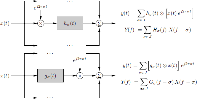
In the special case for which ![]() for some period T0, the system is linear periodically time-variant (LPTV). If J contains only the element σ = 0, then the system is LTI and
for some period T0, the system is linear periodically time-variant (LPTV). If J contains only the element σ = 0, then the system is LTI and ![]() .
.
1.3.3.1 Input/Output Relations
Let us consider two LAPTV systems with impulse-response functions
The (conjugate) cross-correlation of the outputs
is given by (see (Gardner et al. (2006) eq. (3.78)))
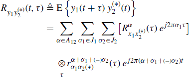
where ![]() denotes convolution with respect to τ, (−) is an optional minus sign that is linked to (*), and
denotes convolution with respect to τ, (−) is an optional minus sign that is linked to (*), and
Thus (see (Napolitano 1995, eqs. (32) and (34)) and (Gardner et al. (2006) eqs. (3.80) and (3.81))), the (conjugate) cyclic cross-correlation function and the (conjugate) cyclic cross-spectrum of the outputs y1(t) and y2(t) are given by
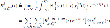
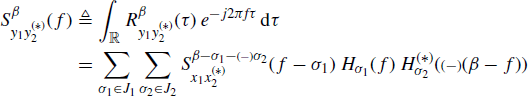
where
(1.118) ![]()
and, in the sums in (1.116) and (1.117), only those σ1 ![]() J1 and σ2
J1 and σ2 ![]() J2 such that
J2 such that ![]()
![]() give nonzero contribution. In the derivation of (1.117), the Fourier transform pair
give nonzero contribution. In the derivation of (1.117), the Fourier transform pair
(1.119) 
is used.
Equations (1.116) and (1.117) can be specialized to several cases of interest. For example, if ![]() , and (*) is conjugation, then we obtain the input-output relations for LAPTV systems in terms of cyclic autocorrelation functions and cyclic spectra:
, and (*) is conjugation, then we obtain the input-output relations for LAPTV systems in terms of cyclic autocorrelation functions and cyclic spectra:
(1.120) ![]()
(1.121) ![]()
where
(1.122) ![]()
By specializing (1.117) to the case ![]() LTI system, and
LTI system, and ![]() we obtain
we obtain
Analogously, by specializing (1.116), we obtain the inverse Fourier transform of both sides of (1.123)
(1.124) ![]()
where, accounting for the Fourier pairs
![]()
![]()
the (conjugate) ambiguity function ![]() can be written in one of the following equivalent forms
can be written in one of the following equivalent forms
(1.125a) 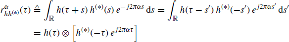
(1.125b) 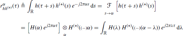
By specializing (1.116) and (1.117) to the case ![]() ,
, ![]() ,
, ![]() ,
, ![]() , so that
, so that ![]() and
and
(1.126) ![]()
we obtain the cyclic cross-statistics of the output and input signals
(1.127) ![]()
(1.128) ![]()
By specializing (1.117) to the case h1 and h2 LTI and (*) absent, for α = 0 we obtain
(1.129) 
(1.130) ![]()
1.3.4 Products of ACS Signals
Let x1(t), x2(t), c1(t), and c2(t) be ACS signals with (conjugate) cross-correlation functions
If x1(t) and x2(t) are statistically independent of c1(t) and c2(t), then their fourth-order joint probability density function factors into the product of the two second-order joint probability densities of x1, x2 and of c1, c2 (Gardner 1987d, 1994), (Brown 1987), and the (conjugate) cross-correlation functions of the product waveforms
(1.133) ![]()
also factors,
(1.134) ![]()
Therefore, the (conjugate) cyclic cross-correlation function and the (conjugate) cyclic cross-spectrum of y1(t) and y2(t) are
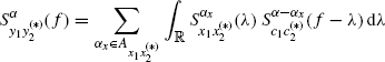
where, in the sums, only those (conjugate) cycle frequencies αx such that ![]() give nonzero contribution. From (1.135) and (1.136), it follows that the set of (conjugate) cycle-frequencies of the (conjugate) cross-correlation of y1(t) and y2(t) is
give nonzero contribution. From (1.135) and (1.136), it follows that the set of (conjugate) cycle-frequencies of the (conjugate) cross-correlation of y1(t) and y2(t) is
(1.137) ![]()
In the special case where c1(t) and c2(t) are almost-periodic functions with (generalized) Fourier series
(1.138) ![]()
then
and
where, in the sum, only those frequencies γ1 such that (−)(α − γ1) ![]() G2 give nonzero contribution. From (1.140) and (1.141) it follows that the set of the (conjugate) cycle-frequencies of the (conjugate) cross-correlation of y1(t) and y2(t) is
G2 give nonzero contribution. From (1.140) and (1.141) it follows that the set of the (conjugate) cycle-frequencies of the (conjugate) cross-correlation of y1(t) and y2(t) is
(1.142) ![]()
In the special case x1 ≡ x2 and c1 ≡ c2, (1.139)–(1.141) reduce to (corrected versions of) (3.93)–(3.95) in (Gardner et al. (2006))). By substituting (1.140) and (1.141) into (1.135) and (1.136), respectively, and making the variable change γ2 = (−)(α − αx − γ1), we get (see (Napolitano 1995, eqs. (46)–(48)))
where, in the sums, only those values of γ1 and γ2 such that ![]() give nonzero contribution. From (1.143) and (1.144), it follows that the set of the (conjugate) cycle-frequencies of the (conjugate) cross-correlation of y1(t) and y2(t) is
give nonzero contribution. From (1.143) and (1.144), it follows that the set of the (conjugate) cycle-frequencies of the (conjugate) cross-correlation of y1(t) and y2(t) is
(1.145) ![]()
1.3.5 Cyclic Statistics of Communications Signals
Cyclostationarity in man-made communications signals is due to signal processing operations used in the construction and/or subsequent processing of signals, such as modulation, sampling, scanning, multiplexing, and coding. Consequently, cycle frequencies are related to parameters such as sinewave carrier frequency, sampling rate, etc. In the following, the cyclic autocorrelation functions and cyclic spectra of two basic communications signals are reported. Further examples can be found in (Gardner 1985, Chapter 12, 1987d), (Gardner et al. 2006) and references therein.
The first signal is the double side-band amplitude-modulated (DSB-AM) signal
(1.146) ![]()
If the modulating process s(t) is WSS, then x(t) is cyclostationary with period 1/(2f0), cyclic autocorrelation functions (Gardner 1985, Chapter 12, 1987d), (Gardner et al. 2006)
(1.147) 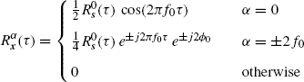
and cyclic spectra
(1.148) 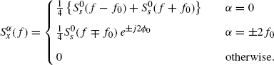
The second signal is the pulse-amplitude-modulated (PAM) signal
(1.149) ![]()
where ![]() is a WSS sequence and q(t) a finite-energy pulse. This PAM signal is cyclostationary with period T0 and (conjugate) cyclic autocorrelation functions and cyclic spectra (Gardner 1985, Chapter 12, 1987d), (Gardner et al. 2006)
is a WSS sequence and q(t) a finite-energy pulse. This PAM signal is cyclostationary with period T0 and (conjugate) cyclic autocorrelation functions and cyclic spectra (Gardner 1985, Chapter 12, 1987d), (Gardner et al. 2006)
for α = m/T0, ![]() , and zero otherwise. In (1.150),
, and zero otherwise. In (1.150),
(1.152) ![]()
and in (1.151) Q(f) is the Fourier transform of q(t).
1.3.6 Higher-Order Statistics
A more complete characterization of stochastic processes can be obtained by considering higher-order statistics. Processes that have almost-periodically time-variant moment and cumulant functions are called higher-order almost-cyclostationary. They have been characterized in the time and frequency domains in (Dandawaté and Giannakis 1994, 1995), (Gardner and Spooner 1994), (Napolitano 1995), (Spooner and Gardner 1994).
A continuous-time complex-valued process x(t) is said to exhibit Nth-order wide-sense cyclostationarity with cycle frequency α ≠ 0, for a given conjugation configuration, if the Nth-order cyclic temporal moment function (CTMF)
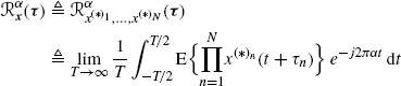
exists and is not zero for some delay vector τ (Gardner and Spooner 1994). In (1.153), ![]()
![]() and
and ![]() are column vectors, and (∗)n represents the nth optional complex conjugation. The process is said to be Nth-order wide-sense almost-cyclostationary if its Nth-order temporal moment function (TMF) is an almost-periodic function of t. Under mild regularity conditions the TMF can be expressed by the (generalized) Fourier series expansion
are column vectors, and (∗)n represents the nth optional complex conjugation. The process is said to be Nth-order wide-sense almost-cyclostationary if its Nth-order temporal moment function (TMF) is an almost-periodic function of t. Under mild regularity conditions the TMF can be expressed by the (generalized) Fourier series expansion
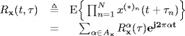
where Ax is a countable set and the sense of equality in (1.154) is one of those discussed in Section 1.2.
The N-fold Fourier transform of the CTMF
which is called the Nth-order cyclic spectral moment function (CSMF), can be written as
(1.156) ![]()
where ![]() is the Dirac delta function,
is the Dirac delta function, ![]() , and primes denote the operator that transforms
, and primes denote the operator that transforms ![]() into
into ![]() . The function
. The function ![]() , referred to as the Nth-order reduced-dimension CSMF (RD-CSMF), can be expressed as the (N − 1)-fold Fourier transform of the Nth-order reduced-dimension CTMF (RD-CTMF) defined as
, referred to as the Nth-order reduced-dimension CSMF (RD-CSMF), can be expressed as the (N − 1)-fold Fourier transform of the Nth-order reduced-dimension CTMF (RD-CTMF) defined as
(1.157) ![]()
For N = 2 and conjugation configuration [xx*], the RD-CTMF is coincident with the cyclic autocorrelation function ![]() , whereas, for conjugation configuration [xx] it is coincident with the conjugate cyclic autocorrelation function
, whereas, for conjugation configuration [xx] it is coincident with the conjugate cyclic autocorrelation function ![]() that can be nonzero only if the signal is noncircular (Picinbono and Bondon 1997), (Schreier and Scharf 2003a,b). It is shown in (Gardner and Spooner 1994) that the RD-CSMF
that can be nonzero only if the signal is noncircular (Picinbono and Bondon 1997), (Schreier and Scharf 2003a,b). It is shown in (Gardner and Spooner 1994) that the RD-CSMF ![]() can contain impulsive terms if the vector f with
can contain impulsive terms if the vector f with ![]() lies on the β-submanifold, i.e., if there exists at least one partition
lies on the β-submanifold, i.e., if there exists at least one partition ![]() of
of ![]() with p > 1 such that each sum
with p > 1 such that each sum ![]() fn is an |μi|th-order cycle frequency of x(t), where |μi| is the number of elements in μi.
fn is an |μi|th-order cycle frequency of x(t), where |μi| is the number of elements in μi.
Note that for second-order statistics, unlike in (1.155), in the complex exponential of double Fourier transforms, an optional minus sign (−) linked to the optional complex conjugation (*) is accounted for (see (1.15), (1.16), and (1.101)).
A well-behaved frequency-domain function that characterizes a signal's higher-order cyclostationarity can be obtained starting from the Nth-order cyclic temporal cumulant function (CTCF), that is, the coefficient
of the (generalized) Fourier-series expansion of the Nth-order temporal cumulant function (Gardner and Spooner 1994)
(1.159a) 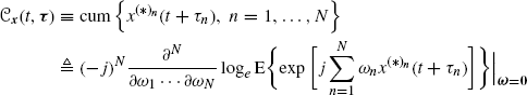
(1.159b) ![]()
where, ![]() ; P is the set of distinct partitions of
; P is the set of distinct partitions of ![]() , each constituted by the subsets
, each constituted by the subsets ![]() ;
; ![]() is the
is the ![]() -dimensional vector whose components are those of x having indices in
-dimensional vector whose components are those of x having indices in ![]() , with
, with ![]() the number of elements in μi. See Section 1.4.2 for a discussion of the definition of (cross-) cumulant of complex random variables and processes.
the number of elements in μi. See Section 1.4.2 for a discussion of the definition of (cross-) cumulant of complex random variables and processes.
The N-fold Fourier transform of ![]() is the Nth-order cyclic spectral cumulant function
is the Nth-order cyclic spectral cumulant function ![]() , which can be written as
, which can be written as ![]() , where the Nth-order cyclic polyspectrum (CP)
, where the Nth-order cyclic polyspectrum (CP) ![]() is the (N − 1)-fold Fourier transform of the reduced-dimension CTCF (RD-CTCF)
is the (N − 1)-fold Fourier transform of the reduced-dimension CTCF (RD-CTCF) ![]() obtained by setting τN = 0 into (1.158). The CP turns out to be a well-behaved function (i.e., it does not contain impulsive terms) under the mild assumption that the time series x(t) and x(t + τ) are asymptotically (τ→ ∞) independent (Section 1.4.1). Moreover, except on a β-submanifold, it is coincident with the RD-CSMF
obtained by setting τN = 0 into (1.158). The CP turns out to be a well-behaved function (i.e., it does not contain impulsive terms) under the mild assumption that the time series x(t) and x(t + τ) are asymptotically (τ→ ∞) independent (Section 1.4.1). Moreover, except on a β-submanifold, it is coincident with the RD-CSMF ![]() .
.
Higher-order cyclostationarity can be exploited when the second-order cyclostationarity features of the signal of interest are zero or weak. Moreover, since they provide a more complete characterization of signals, higher-order cyclostationarity is suitable to be used in modulation format classification and cognitive radio (Spooner and Nicholls 2009).
1.3.7 Cyclic Statistic Estimators
Consistent estimates of second-order statistical functions of an ACS stochastic process can be obtained provided that the stochastic process has finite or “effectively finite” memory. Such a property is generally expressed in terms of mixing conditions or summability of second-and fourth-order cumulants. Under such mixing conditions, the cyclic correlogram is a consistent estimator of the cyclic autocorrelation function. Moreover, a properly normalized version of the cyclic correlogram is asymptotically zero-mean complex Normal as the observation interval approaches infinity. In the frequency domain, the cyclic periodogram is an asymptotically unbiased but not consistent estimator of the cyclic spectrum. However, under appropriate conditions, the frequency-smoothed cyclic periodogram is a consistent estimator of the cyclic spectrum. Moreover, a properly normalized version of the frequency-smoothed cyclic periodogram is asymptotically zero-mean complex Normal as the observation interval approaches infinity and the width of the frequency-smoothing window approaches zero. In addition, the time-smoothed cyclic periodogram is asymptotically equivalent to the frequency-smoothed cyclic periodogram.
Consistent estimators of (conjugate) cyclic autocorrelation function and cyclic spectrum are proposed and analyzed in (Hurd and Le![]() kow 1992a,b), (Dandawaté and Giannakis 1994, 1995), (Dehay 1994), (Dehay and Hurd 1994), (Hurd and Miamee 2007), and references therein. These results can be obtained by specializing to ACS processes the results presented in Chapters 2 and 4. Higher-order cyclic statistic estimators are presented in (Dandawaté and Giannakis 1994, 1995), and (Napolitano and Spooner 2000).
kow 1992a,b), (Dandawaté and Giannakis 1994, 1995), (Dehay 1994), (Dehay and Hurd 1994), (Hurd and Miamee 2007), and references therein. These results can be obtained by specializing to ACS processes the results presented in Chapters 2 and 4. Higher-order cyclic statistic estimators are presented in (Dandawaté and Giannakis 1994, 1995), and (Napolitano and Spooner 2000).
1.3.8 Discrete-Time ACS Signals
ACS processes, such as WSS processes, can also be defined in discrete time. The definitions are similar to those in continuous time with the obvious modifications (Gladyshev 1961), (Gardner 1985, 1994), (Dandawaté and Giannakis 1994), (Napolitano 1995), (Giannakis 1998), (Gardner et al. 2006).
Let us consider a discrete-time complex-valued stochastic process ![]() , with abbreviated notation xd(n) when this does not create ambiguity. The stochastic process xd(n) is said to be second-order almost-cyclostationary in the wide sense (Gardner 1985) if its mean value E{xd(n)} and its (conjugate) autocorrelation function
, with abbreviated notation xd(n) when this does not create ambiguity. The stochastic process xd(n) is said to be second-order almost-cyclostationary in the wide sense (Gardner 1985) if its mean value E{xd(n)} and its (conjugate) autocorrelation function
(1.160) ![]()
with subscript ![]() , are almost-periodic functions of the discrete-time parameter n. Thus, under mild regularity assumptions the (conjugate) autocorrelation function can be expressed by the (generalized) Fourier series
, are almost-periodic functions of the discrete-time parameter n. Thus, under mild regularity assumptions the (conjugate) autocorrelation function can be expressed by the (generalized) Fourier series
where
(1.162) ![]()
is the (conjugate) cyclic autocorrelation function at (conjugate) cycle frequency ![]() and
and
(1.163) ![]()
is a countable set. Note that the (conjugate) cyclic autocorrelation function ![]() is periodic in
is periodic in ![]() with period 1. Thus, the sum in (1.161) can be equivalently extended to the set
with period 1. Thus, the sum in (1.161) can be equivalently extended to the set ![]()
![]() .
.
In general, the set ![]() (or
(or ![]() ) depends on the optional complex conjugation (*) and possibly contains incommensurate cycle frequencies
) depends on the optional complex conjugation (*) and possibly contains incommensurate cycle frequencies ![]() and cluster points. In the special case where
and cluster points. In the special case where ![]()
![]() for some integer N0, the (conjugate) autocorrelation function
for some integer N0, the (conjugate) autocorrelation function ![]() is periodic in n with period N0. If also E{xd(n)} is periodic with period N0, the process x(n) is said to be cyclostationary in the wide sense. If N0 = 1 then x(n) is wide-sense stationary.
is periodic in n with period N0. If also E{xd(n)} is periodic with period N0, the process x(n) is said to be cyclostationary in the wide sense. If N0 = 1 then x(n) is wide-sense stationary.
Let
(1.164) ![]()
be the stochastic process obtained from Fourier transformation (in a generalized sense (Gelfand and Vilenkin 1964, Chapter 3)) of the ACS process x(n). By using (1.161), in the sense of distributions, it can be shown that (Hurd 1991)
where
(1.166) ![]()
is the (conjugate) cyclic spectrum at (conjugate) cycle frequency ![]() . The cyclic spectrum
. The cyclic spectrum ![]() is periodic in both ν and
is periodic in both ν and ![]() with period 1.
with period 1.
In (Gladyshev 1961) and (Dehay 1994), it is shown that discrete-time cyclostationary processes are harmonizable.
1.3.9 Sampling of ACS Signals
Let
(1.167) ![]()
be the discrete-time process obtained by uniformly sampling with period Ts = 1/fs the continuous-time ACS signal xa(t) with Loève bifrequency spectrum (see (1.94))
where subscript ![]() . Accounting for the relationship between the Fourier transform Xa(f) of the continuous-time signal xa(t) and the Fourier transform X(ν) of the discrete-time sampled signal x(n) (Lathi 2002, Section 9.5)
. Accounting for the relationship between the Fourier transform Xa(f) of the continuous-time signal xa(t) and the Fourier transform X(ν) of the discrete-time sampled signal x(n) (Lathi 2002, Section 9.5)
(1.169) ![]()
we have the following result.
Lemma 1.3.1 Aliasing Formula for the Loève Bifrequency Spectrum of a Sampled ACS Signal.
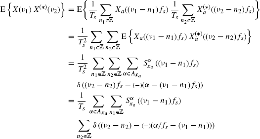
where, in the last equality, the scaling property of the Dirac delta ![]() is used (Zemanian 1987, Section 1.7).
is used (Zemanian 1987, Section 1.7). ![]()
Corollary 1.3.2 From (1.170), it follows that the discrete-time signal ![]() obtained by uniformly sampling a continuous-time ACS signal xa(t) is a discrete-time ACS signal. In fact, its Loève bifrequency spectrum has support concentrated on lines with slope ±1 in the bifrequency plane (ν1, ν2) and can be written in the form (1.165).
obtained by uniformly sampling a continuous-time ACS signal xa(t) is a discrete-time ACS signal. In fact, its Loève bifrequency spectrum has support concentrated on lines with slope ±1 in the bifrequency plane (ν1, ν2) and can be written in the form (1.165).
The countable set ![]() in (1.165) is linked to
in (1.165) is linked to ![]() by the relationships
by the relationships
with mod 1 denoting the modulo 1 operation with values in (− 1/2, 1/2] and equality can hold in (1.172) only if xa(t) is not strictly bandlimited. ![]()
The (conjugate) cyclic spectrum and the (conjugate) cyclic autocorrelation function of x(n) are given in the following result.
Lemma 1.3.3 Aliasing Formulas for Cyclic Statistics of ACS Signals (Izzo and Napolitano 1996), (Napolitano 1995).
where x ![]() [xx(*)].
[xx(*)]. ![]()
Assumption 1.3.4 The continuous-time process xa(t) is strictly band-limited, i.e., ![]()
![]() (Gardner et al. (2006) Section 3.8).
(Gardner et al. (2006) Section 3.8).
Lemma 1.3.5 Support of the (Conjugate) Cyclic Spectrum. Under Assumption 1.3.4 (xa(t) strictly band-limited), it results that (Gardner et al. (2006) eqs. (3.100) and (3.111), Figure 1.1):
Therefore,
(1.177) ![]()
Moreover, in (1.168) we have
![]()
Consequently, under Assumption 1.1 (xa(t) strictly band-limited), and accounting for (1.176a), the support of the replica with n1 = n2 = 0 in the aliasing formula (1.170) is given by
(1.179a) 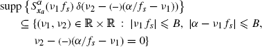
Theorem 1.3.6 ACS Signals: Sampling Theorem for the Discrete-Time Loève Bifrequency Spectrum. Under Assumption 1.3.4 and for fs ≥ 4B, it results in

Moreover,
Proof: Replicas in (1.170) are separated by 1 in both ν1 and ν2 variables. Thus, from (1.179b) it follows that B/fs ≤ 1/2, that is,
is a sufficient condition such that replicas do not overlap. Note that, however, (1.182) does not assure that the mappings ![]() and
and ![]() in
in
holds ![]() and
and ![]() . For example, for (*) present and α = − B, equality (1.183) holds only for ν1
. For example, for (*) present and α = − B, equality (1.183) holds only for ν1 ![]() [− 1/2, 0] and not for ν1
[− 1/2, 0] and not for ν1 ![]() [0, 1/2]. In fact, for ν1
[0, 1/2]. In fact, for ν1 ![]() [0, 1/2] the density of the replica with n1 = 0, n2 = 1 should be present in the right-hand side of (1.183).
[0, 1/2] the density of the replica with n1 = 0, n2 = 1 should be present in the right-hand side of (1.183).
In contrast, condition ![]() , that is,
, that is,
assures in (1.179b)
(1.185) ![]()
and, consequently, the mappings ![]() and
and ![]() in (1.183) hold
in (1.183) hold ![]() and ∀ν1
and ∀ν1 ![]() [− 1/2, 1/2). Moreover, (1.180) holds. Finally, note that the effect of sampling at two times the Nyquist rate (see (1.184)) leads also to (1.181).
[− 1/2, 1/2). Moreover, (1.180) holds. Finally, note that the effect of sampling at two times the Nyquist rate (see (1.184)) leads also to (1.181).
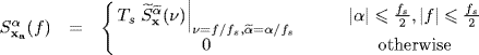
Theorem 1.3.7 Sampling Theorem for Cyclic Statistics of ACS Signals (Napolitano 1995), (Izzo and Napolitano 1996). Under Assumption 1.1 and for fs ≥ 4B, the result is
(1.186a) ![]()
(1.186b) 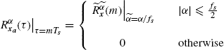
(1.188a) ![]()
where ![]() and x = [xx(*)]. By Fourier transforming both sides in (1.187) we get the following expression for the cyclic spectra of a strictly band-limited signal
and x = [xx(*)]. By Fourier transforming both sides in (1.187) we get the following expression for the cyclic spectra of a strictly band-limited signal
(1.189) ![]()
which is equivalent to (1.188b). ![]()
1.3.10 Multirate Processing of Discrete-Time ACS Signals
Expansion and decimation are linear time-variant transformations that are not almost-periodically time-variant. Consequently, the results of Section 1.3.3 cannot be used. In Section 4.3.1, it is observed that expansion and decimation belong to the class of linear time-variant systems that can be classified as deterministic in the FOT probability sense. These systems transform input ACS signals into output ACS signals with different almost-cyclostationarity characteristics (Sathe and Vaidyanathan 1993), (Izzo and Napolitano 1998b), (Akkarakaran and Vaidyanathan 2000). In contrast, in Section 4.10, it is shown that cross-statistics of signals generated with different rates by the same ACS signal give rise to signals that are jointly SC.
Results on multirate processing of discrete-time ACS processes are obtained as special cases of results on multirate processing of spectrally correlated processes in Section 4.10.
1.3.11 Applications
The existence of consistent estimators for the cyclic statistics is one of the main motivations for many applications of cyclostationarity in several fields such as communications, circuits, systems and control, acoustics, mechanics, econometrics, biology, and astronomy (Gardner et al. 2006). Applications in mechanics and vibroacoustic signal analysis are discussed in (Antoni 2009) and references therein.
In communications and radar/sonar applications, cyclostationarity properties can be used to design signal selective detection and estimation algorithms. In fact, in the case of additive noise uncorrelated with the signal of interest (SOI), if the SOI does not share at least one cycle frequency, say α0, with the disturbance, then the cyclic autocorrelation function of the SOI plus noise at α0 is coincident with the cyclic autocorrelation function of the SOI alone. Therefore, detection or estimation algorithms operating at α0 are potentially immune to the effects of noise and interference, provided that a sufficiently long observation interval is adopted to estimate the cyclic statistics (Gardner 1985, 1987d), (Gardner and Chen 1992), (Chen and Gardner 1992), (Gardner and Spooner 1992, 1993), (Flagiello et al. 2000). In (Gardner et al. 2006) and references therein, applications of cyclostationarity for interference tolerant channel identification and equalization, signal detection and classification, source separation, periodic autoregressive (AR) and autoregressive moving-average (ARMA) modeling and prediction, are described. The spectral line regeneration property of ACS signal can be exploited for synchronization purposes (Gardner 1987d).
Cyclostationarity properties can be suitably exploited in minimum mean-square error (MMSE) linear filtering or Wiener filtering. If the useful signal, the data, and the disturbance signal are singularly and jointly ACS, then it can be shown that the optimum linear filter is linear almost-periodically time variant. By exploiting the spectral correlation property of ACS signals, the optimum filter cancels the spectral bands of the useful signal which are corrupted by noise and then reconstructs these bands exploiting the spectral components of the useful signal that are noise-free and correlated with the canceled bands (Gardner 1993). This MMSE filtering procedure is referred to as cyclic Wiener filtering or frequency shift (FRESH) filtering. It provides significant performance improvement with respect to the classical Wiener filtering that assumes a stationary model for the involved signals.
Second-and higher-order cyclostationarity properties can be exploited for modulation format classification. The classification is performed by comparing estimated second-and higher-order cyclic features of the received signal with those stored in a catalog (Spooner and Gardner 1994), (Spooner and Nicholls 2009).