
3.11 Proofs for Section 2.6.3 “Asymptotic Results as N→ ∞ and Ts → 0′′
3.11.1 Proof of Lemma 2.6.12
Condition (2.209) holding uniformly w.r.t. τ assures that Assumption 2.6.11 is verified. The numbers Mp, possibly depending on ![]() , are independent of Ts. Under Assumption 2.6.11, the Weierstrass M-test (Johnsonbaugh and Pfaffenberger 2002, Theorem 62.6) assures the uniform convergence of the series of functions of Ts
, are independent of Ts. Under Assumption 2.6.11, the Weierstrass M-test (Johnsonbaugh and Pfaffenberger 2002, Theorem 62.6) assures the uniform convergence of the series of functions of Ts
Therefore, the limit operation can be interchanged with the infinite sum
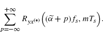
(3.207) 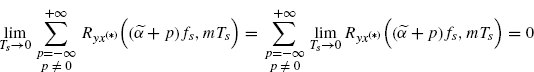
where, in the second equality the sufficient condition (2.209) for Assumption 2.6.11 is used.
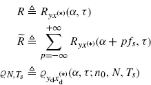
3.11.2 Proof of Theorem 2.6.13 Mean-Square Consistency of the Discrete-Time Cyclic Cross-Correlogram
From Lemma 2.6.12 we have
(3.208) 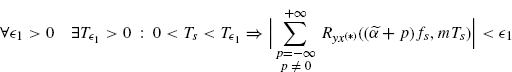
(not necessarily uniformly with respect to ![]() and m).
and m).
From Theorems 2.6.4 and 2.6.5 it follows that, for every fixed Ts, ![]() , and m,
, and m,
that is,
(3.210) 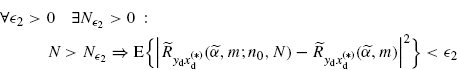
Therefore, for ![]() and
and ![]() we have
we have
(3.211) 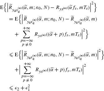
with ![]() 1 and
1 and ![]() 2 arbitrarily small. Note that the limit is not necessarily uniform in
2 arbitrarily small. Note that the limit is not necessarily uniform in ![]() .
.
Equation (3.209) holds for fixed (and finite) Ts > 0. Therefore, in (2.211) we have that first N→ ∞ and then Ts → 0. This order of the two limits is in agreement with the result of (Dehay 2007) where Ts = N−δ with 0 < δ < 1.
3.11.3 Noninteger Time-Shift
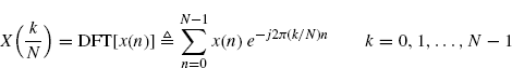
Let us consider a discrete-time signal x(n) with Fourier transform X(ν).
(3.212) 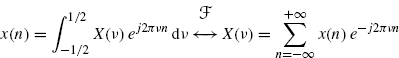
Definition 3.11.1 The time-shifted version of x(n) with noninteger time-shift μ is defined as
(3.213) 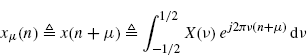
![]()
Fact 3.11.2 If x(n) is a finite N-length sequence defined for n ![]() {0, 1, ..., N − 1}, the time-shifted version of x(n) with noninteger time-shift μ, can be expressed by the exact interpolation formula
{0, 1, ..., N − 1}, the time-shifted version of x(n) with noninteger time-shift μ, can be expressed by the exact interpolation formula
In (3.214),
is the discrete Fourier transform (DFT) of x(n) and
(3.216a) 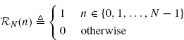
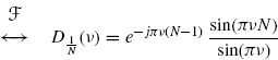
with ![]() referred to as Dirichlet kernel. According to Definition 3.11.1, we have
referred to as Dirichlet kernel. According to Definition 3.11.1, we have
Alternatively, the time-shifted version of x(n) with noninteger time-shift μ, can be expressed by the exact interpolation formula
(3.218) 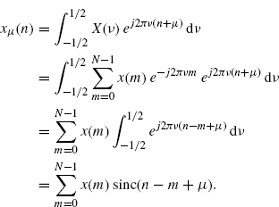
![]()
3.11.4 Proof of Theorem 2.6.16 Asymptotic Expected Value of the Hybrid Cyclic Cross-Correlogram
Use a simple modification of Lemma 2.6.12 with mTs replaced by τ and then use (2.217a)
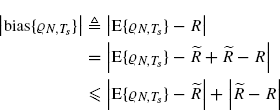
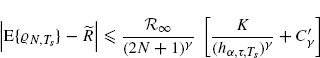
3.11.5 Proof of Theorem 2.6.17 Rate of Convergence of the Bias of the Hybrid Cyclic Cross-Correlogram
Let us consider the set
defined in (2.222). Since ![]() is assumed to be finite and the functions αk(τ) are bounded for finite τ, the sampling period Ts can be chosen sufficiently small such that
is assumed to be finite and the functions αk(τ) are bounded for finite τ, the sampling period Ts can be chosen sufficiently small such that
(3.220) ![]()
that is, mod fs is not necessary in the definition (3.219). Moreover, if ![]() , then αk(τ) ≠ α. Thus, for Ts sufficiently small (depending on α and τ) the result is that
, then αk(τ) ≠ α. Thus, for Ts sufficiently small (depending on α and τ) the result is that
In addition, since ![]() is finite, for Ts sufficiently small (α − αk(τ))Ts = 0 only if α = αk(τ). Therefore, for Ts sufficiently small (depending on α and τ) we have
is finite, for Ts sufficiently small (α − αk(τ))Ts = 0 only if α = αk(τ). Therefore, for Ts sufficiently small (depending on α and τ) we have
(3.222) 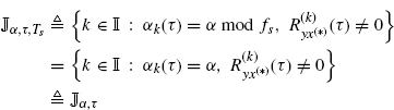
finite set not depending on Ts. Consequently,
(3.223) ![]()
Since for Ts small we have that ![]() finite set independent of Ts, with regard to the quantity
finite set independent of Ts, with regard to the quantity ![]() defined in (2.223), for Ts small we have
defined in (2.223), for Ts small we have
(3.224) 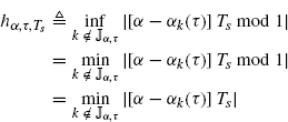
where in the second equality inf is substituted by min since ![]() (and also
(and also ![]() ) is finite, and the third equality holds for Ts sufficiently small (depending on α and τ) such that (3.221) holds. Therefore,
) is finite, and the third equality holds for Ts sufficiently small (depending on α and τ) such that (3.221) holds. Therefore,
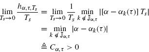
(3.225) 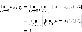
provided that the functions αk(τ) are bounded for finite τ. In the second equality, lim and min operations can be interchanged since min is over a finite set not depending on Ts (in general, lim and inf operations cannot be inverted if inf is over an infinite set). In addition,
Let us define for notation simplicity
It results that
Under the assumption of finite ![]() , Assumption 2.6.11 is verified and the thesis of Lemma 2.6.12 is also verified since in the right-hand side of
, Assumption 2.6.11 is verified and the thesis of Lemma 2.6.12 is also verified since in the right-hand side of
(3.228) 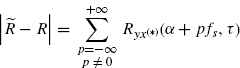
the sum is identically zero for Ts sufficiently small (depending on τ), that is, for fs sufficiently large so that, for fixed τ,
(3.229) ![]()
where the maximum exists since the number of lag-dependent cycle frequencies is finite and each function αk(τ) is assumed to be bounded for finite τ.
From the counterpart for the H-CCC of Theorem 2.6.7, it follows that (see (3.199))
where ![]() and
and
(3.231) 
Consequently, from (3.226), (3.227), and (3.230), we have
(3.232) 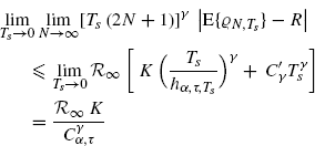
where ![]() and the order of the two limits cannot be inverted.
and the order of the two limits cannot be inverted.
3.11.6 Proof of Theorem 2.6.18 Asymptotic Covariance of the Hybrid Cyclic Cross-Correlogram
Let us consider the limit
(3.233) 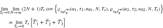
where ![]() ,
, ![]() , and
, and ![]() are defined in (2.196), (2.197), and (2.198), respectively, with the replacements
are defined in (2.196), (2.197), and (2.198), respectively, with the replacements ![]() and
and ![]() .
.
As regards the term ![]() , we have
, we have
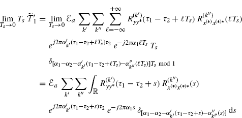
with the right-hand side coincident with ![]() defined in (2.147). In (3.234), we used the fact that if αk(τ) are bounded and
defined in (2.147). In (3.234), we used the fact that if αk(τ) are bounded and ![]() and
and ![]() are finite sets, for Ts sufficiently small, one has
are finite sets, for Ts sufficiently small, one has
(3.235) 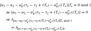
In addition, the integrand function has been assumed to be Riemann integrable.
Note that the right-hand side of (3.234) can be nonzero only if ![]() in a set of values of s with positive Lebesgue measure.
in a set of values of s with positive Lebesgue measure.
Analogous results hold for terms ![]() , and
, and ![]() .
.
3.11.7 Proof of Lemma 2.6.19 Rate of Convergence to Zero of Cumulants of Hybrid Cyclic Cross-Correlograms
From (3.203) it follows that
where the sums over ri, i = 1, ..., k − 1, and n in the second term range over sets {ri,min, ..., ri,max} and {nmin, ..., nmax} with extremes ri,min, ri,max, nmin, nmax depending on N and such that, as N→ ∞, ri,min and nmin approach −∞ and ri,max and nmax approach +∞.
The rhs of (3.236) does not depend on ![]() , mi. Therefore, the same inequality holds by replacing in the lhs
, mi. Therefore, the same inequality holds by replacing in the lhs ![]() with
with ![]() and we also have
and we also have
(3.237) 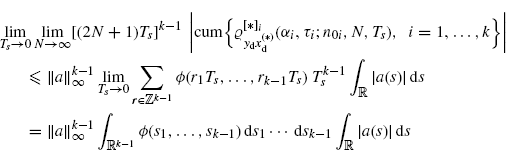
Thus, for k ![]() 2 and
2 and ![]() > 0, we obtain (2.230), where the order of the two limits cannot be interchanged (that is, NTs→ ∞).
> 0, we obtain (2.230), where the order of the two limits cannot be interchanged (that is, NTs→ ∞).
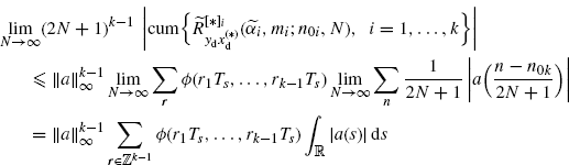
Note that the (k − 1)-dimensional Riemann sum in the second line converges to the (k − 1)-dimensional Riemann integral in the third line if the Riemann-integrable function ϕ is sufficiently regular. In fact, the limit as Ts → 0 of the infinite sum in the second line is not exactly the definition of a Riemann integral over an infinite (k − 1)-dimensional interval. However, the function ϕ in Assumption 2.6.8 can always be chosen such that this Riemann integral exists.
![]()
3.11.8 Proof of Theorem 2.6.20 Asymptotic Joint Normality of the Hybrid Cyclic Cross-Correlograms
By following the guidelines of the proof of Theorem 2.6.10, let
(3.238) 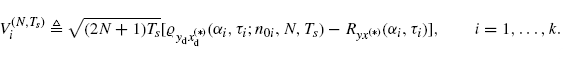
From Theorem 2.6.17 holding for γ > 1 (or γ = 1 if a(t) = rect(t)), we have
(3.239) ![]()
From Theorem 2.6.18, we have that
is finite. From Theorem 3.13.3, we have that
is finite. From Lemma 2.6.19 with ![]() and k
and k ![]() 3, we have
3, we have
(3.240) ![]()
Thus, according to the results of Section 1.4.2, for every fixed αi, τi, n0i the random variables ![]() , i = 1, ..., k, are asymptotically (N→ ∞ and Ts → 0 with NTs→ ∞) zero-mean jointly complex Normal (Picinbono 1996; van den Bos 1995).
, i = 1, ..., k, are asymptotically (N→ ∞ and Ts → 0 with NTs→ ∞) zero-mean jointly complex Normal (Picinbono 1996; van den Bos 1995).